


“To Predict” Is Useful - But Is It Enough?
As a data scientist, you’ve likely mastered machine learning, but have you tapped into the potential of mathematical optimization? Better yet, have you ever combined these two powerful techniques in a single project?
This post is designed to:
- Inspire you with real-world applications.
- Challenge you to think beyond standalone ML models.
- Equip you with insights for problems where optimization + ML outperform either approach alone.
While machine learning excels at predictions, many business problems demand actionable decisions, where optimization shines. Knowing when (and how) to merge these disciplines can transform good solutions into game-changing ones. Let’s explore how to bridge the gap between predictive power and optimal decision-making.
Combining machine learning and mathematical optimization offers enormous potential, but it requires caution. While ML is effective at capturing complex patterns from data, it rarely answers the central decision-making question: what to do with those predictions? That’s where optimization comes in, turning forecasts into actionable decisions within real-world operational constraints. On the other hand, optimization models rely on well-defined parameters and structures, often difficult to obtain and model in dynamic environments. ML can address this limitation by providing estimates, distributions, or even entire functions as inputs to prescriptive models.
However, integrating these approaches is not trivial. Inaccurate predictive models can compromise the entire decision chain. Optimized solutions based on biased forecasts risk being unfeasible in practice. That’s why the quality of integration between predictions and decisions matters more than the standalone performance of each model. Truly leveraging this combination requires more than just applying tools. It demands a deep understanding of the problem, clarity about each method’s role, and discipline to jointly validate results. When well-executed, this integration turns data into a sustainable competitive advantage.
Understanding the Strengths and Limitations of Each Approach
Machine learning and mathematical optimization each excel in different scenarios, but they also come with inherent constraints. ML models can struggle with concept drift when data distributions shift significantly, requiring costly retraining. Optimization models demand precise problem formulation and struggle with unstructured inputs that ML handles effortlessly. Additionally, large-scale optimization problems often require expensive commercial solvers.
The choice between techniques depends on your problem:
- Machine learning shines for pattern recognition, similarity analysis, and predictive tasks like weather forecasting
- Optimization dominates when making operational decisions - scheduling, resource allocation, or cost minimization
Selecting the appropriate methodology upfront is crucial. Misapplying these tools leads to wasted effort, while proper alignment creates elegant solutions. The most powerful applications often emerge when we strategically combine both approaches.
Analyzing Avocado Market Trends with Real-World Data
Our analysis leverages actual sales data from the Hass Avocado Board (HAB), an organization committed to promoting avocado consumption across the United States. The dataset provides comprehensive weekly records of avocado prices and sales volumes across multiple years.
To ensure a robust historical perspective, we’ve combined two data sources: the primary dataset obtained directly from HAB covering 2019 through 2022, supplemented by an earlier dataset from Kaggle spanning 2015 to 2018. This combined approach allows for more meaningful trend analysis over an extended period.
The dataset contains detailed weekly entries documenting sales quantities and average prices, segmented by geographic region and avocado type. While the data includes both conventional and organic varieties, our current analysis focuses specifically on conventional avocados. The geographic coverage spans eight major U.S. regions: the Great Lakes, Midsouth, Northeast, Northern New England, South Central, Southeast, West, and Plains.
With the data sources established, our first step involves loading this information into a structured format for analysis. The dataset will be imported into a Pandas dataframe, providing the foundation for subsequent exploration and modeling. This initial preparation phase is crucial for ensuring data quality and accessibility as we progress through our analytical workflow. The Hass Avocado Board, the primary source of data on the U.S. avocado market, identifies three critical factors that influence prices:
- The balance between regional supply and demand, by consumption peaks during specific events like the Super Bowl.
- Weather conditions in key producing regions, such as droughts in California or storms in Mexico.
- The operational costs involved in transportation and importation, directly impacted by fuel prices and tariff policies.
The application of Machine Learning techniques provides a robust solution to this complex pricing equation. By processing historical sales data, production volumes, and external variables (such as climate and economic indicators).
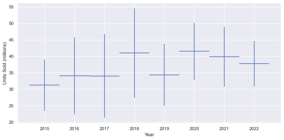
The data reveals a gradual upward trend in avocado sales over time, though growth remains modest overall. Notably, we observe a significant deviation from this pattern in 2019, corresponding to the well-documented 2019 avocado shortage. This supply crisis had substantial market impacts, with:
- A pronounced dip in sales volume
- Retail prices nearly doubled during the shortage period
This event serves as a valuable case study in how supply shocks can disrupt established consumption patterns. The clear correlation between reduced availability and both higher prices and lower sales volumes demonstrates the fundamental relationship between these market factors. Let’s see the sales trends within a year.
We see a Super Bowl peak in February and a Cinco de Mayo peak in May. In that way let’s take a look in the avocado price correlation
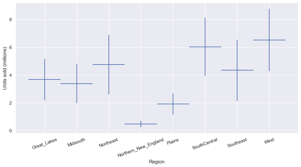
As expected, the sales quantity has a negative correlation with the price per avocado. The sales quantity has a positive correlation with the year and season, being a peak season. Let’s take a look at how the sales differ among the different regions. This will determine the number of avocados that we want to supply to each region.
A Regression Analysis of Market Drivers
The observed trends in avocado sales suggest a strong dependency on price, time, geography, and seasonality. To quantify these relationships, we propose a linear regression model that predicts demand as a function of these key variables. This approach allows us to measure the individual impact of each factor while providing an interpretable framework for forecasting.
At its core, the model treats demand as a linear combination of predictors: price acts as a primary continuous variable, expected to inversely affect sales; region is incorporated through categorical encoding to capture fixed market differences; year accounts for long-term trends in avocado consumption; and a binary seasonal indicator differentiates peak demand periods from baseline activity. The regression coefficients represent the marginal effect of each variable, translating business observations into actionable parameters.
To ensure statistical rigor, we partition the data into training and testing sets, reserving 20% of observations for out-of-sample validation. This guards against overfitting and provides an honest assessment of predictive performance. The model’s adequacy will be evaluated through standard metrics including, R-squared for goodness-of-fit and root mean squared error for prediction accuracy, while residual analysis will verify whether linear assumptions hold across different market segments.
This foundational model serves multiple purposes: it establishes a performance benchmark for more complex algorithms, offers transparent insights into demand drivers, and creates a framework for what-if scenario analysis. Future refinements could introduce interaction terms or nonlinear transformations, but the current specification already provides a robust tool for understanding avocado market dynamics. The simplicity and interpretability of linear regression make it particularly valuable for business decision-making, where understanding why a model predicts certain outcomes is often as important as the predictions themselves.
So, trends observed motivate us to construct a prediction model for sales using the independent variables- price, year, region, and seasonality. Henceforth, the sales quantity will be referred to as the predicted demand. Let us now construct a linear regressor for the demand. Note that the region is a categorical variable. The linear regressor can be mathematically expressed as:
The linear regressor can be mathematically expressed as:
\[demand = \beta_0 + \beta_1 * price + \sum\limits_{region} \beta^{region}_3 * \mathbb{1}(region) + \beta_4 w_{year}*year + \beta_5 * \mathbb{1}(peak).\]Here, the \(\beta\) values are weights (or “coefficients”) that have to be learned from the data. Note that the notation \(\mathbb{1}(region)\) is an indicator function that takes the value \(1\) for each region in the summation. The value of \(\mathbb{1}(peak)\) is \(1\) if we consider the peak season.
Knowing how the price of an avocado affects the demand, how can we set the optimal avocado price?
Why Modeling Refinement Beats Premature Pipelines
We don’t want to set the price too high, since that could drive demand and sales down. At the same time, setting the price too low could be sub-optimal when maximizing revenue. So what is the sweet spot?
On the distribution logistics, we want to make sure that there are enough avocados across the regions. We can address these considerations in a mathematical optimization model. An optimization model finds the best solution according to an objective function such that the solution satisfies a set of constraints. Here, a solution is expressed as a vector of real values or integer values called decision variables. Constraints are a set of equations or inequalities written as a function of the decision variables.
At the start of each week, assume that the total number of available products is finite. This quantity needs to be distributed to the various regions while maximizing net revenue. So there are two key decisions - the price of an avocado in each region, and the number of avocados allocated to each region.
Let us now define some input parameters and notations used for creating the model. The subscript \(r\) will be used to denote each region.
Input Parameters
- \(R\): set of regions,
- \(d(p,r)\): predicted demand in region \(r\in R\) when the avocado per product is \(p\),
- \(B\): available avocados to be distributed across the regions,
- \(c_{waste}\): cost per wasted avocado,
- \(c^r_{transport}\): cost of transporting an avocado to the region \(r \in R\),
- \(a^r_{min},a^r_{max}\): minimum and maximum price per avocado for region \(r \in R\),
- \(b^r_{min},b^r_{max}\): minimum and maximum number of avocados allocated to the region \(r \in R\),
Decision Variables
Let us now define the decision variables. In our model, we want to store the price and number of avocados allocated to each region. We also want variables that track how many avocados are predicted to be sold and how many are predicted to be wasted. The following notation is used to model these decision variables, indexed for each region \(r\).
- \(p_r\): the price of an avocado (in dollars) in the region \(r\),
- \(x_r\): the number of products of avocados supplied to the region \(r\),
- \(s_r = \min \{x_r,d_r(p_r)\}\): the predicted number of avocados sold in the region \(r\),
- \(w_r = x_r - s_r\): the predicted number of avocados wasted in the region \(r\)
Add the Supply Constraint
We now introduce the constraints. The first constraint is to make sure that the total number of avocados supplied is equal to \(B\), which can be mathematically expressed as follows.
\[\begin{align*} \sum_{r} x_r &= B \end{align*}\]Add Constraints That Define Sales Quantity
As a quick reminder, the sales quantity is the minimum of the allocated quantity and the predicted demand, i.e., \(s_r = \min \{x_r,d_r(p_r)\}\) This relationship can be modeled by the following two constraints for each region $r$.
\[\begin{align*} s_r &\leq x_r \\ s_r &\leq d(p_r,r) \end{align*}\]Add the Wastage Constraints
Finally, we should define the predicted wastage in each region, given by the supplied quantity that is not predicted to be sold. We can express this mathematically for each region \(r\).
\[\begin{align*} w_r &= x_r - s_r \end{align*}\]Set the Objective
Finally, the goal is to maximize the net revenue, which is the product of price and quantity, minus costs over all regions. This model assumes the purchase costs are fixed (since the amount \(B\) is fixed) and are therefore not incorporated.
Using the defined decision variables, the objective can be written as follows.
\[max \sum_{r} (p_r * s_r - c_{waste} * w_r - c^r_{transport} * x_r)\]So the final model can be written as follows:
\[\begin{align} \max \quad & \sum_{r} (p_r \cdot s_r - c_{\text{waste}} \cdot w_r - c^r_{\text{transport}} \cdot x_r) \tag{1} \\ \text{s.t.} \quad & \sum_{r} x_r = B \tag{2} \\ s_r &\leq x_r \tag{3} \\ s_r &\leq d(p_r,r) \tag{4} \\ w_r &= x_r - s_r \tag{5} \\ \end{align}\]Ok! We have added the decision variables, objective function, and constraints to the model. The model is ready to be solved. Let’s recap what we have done so far.
Until now, he has set dependency relationship between avocado sales (\(g(x)=y\)) and dependent variables, and also we established a mathematical model to define how to address the avocado demand. In other words, a regression model may predict the demand of certain products as a function of their prices and marketing budgets, among other features. But, more than that, we are interested in being able to build optimization models that embed the regression so that the inputs of the regression are decision variables, and the predicted demand can be satisfied. Let’s solve it
Solve the problem
We have now fully constructed our optimization model by defining all decision variables, the objective function, and the necessary constraints. With these components in place, the model is prepared for solving. However, before initiating the solution process, we need to explicitly specify the model type to the solver. By default, most optimization solvers assume a linear programming framework where both the objective function and constraints are linear relationships. Since our model may involve more complex relationships, we should verify and configure the appropriate model type settings accordingly.
This step ensures the solver applies the most suitable algorithms and techniques for our specific problem structure, whether it involves linear, quadratic, or more general nonlinear relationships. Proper model classification at this stage can significantly impact both the solution accuracy and computational efficiency. In our model, the objective is quadratic since we take the product of price and the predicted sales, both of which are variables.
| Region | Price | Allocated | Sold | Wasted | Pred_demand |
|---|---|---|---|---|---|
| Great_Lakes | 1.663872 | 3.446414 | 3.446414 | 1.000000e-08 | 3.446414 |
| Midsouth | 1.508809 | 5.272290 | 3.545445 | 1.726845e+00 | 3.545445 |
| Northeast | 2.000000 | 4.138685 | 4.138685 | 1.000000e-08 | 4.138685 |
| Northern_New_England | 1.441157 | 0.917984 | 0.917984 | 0.000000e+00 | 0.917984 |
| SouthCentral | 2.000000 | 4.419478 | 4.419478 | 1.000000e-08 | 4.419478 |
| Southeast | 1.746370 | 3.848598 | 3.848598 | 2.000000e-08 | 3.848598 |
| West | 2.000000 | 5.307465 | 5.307465 | 2.000000e-08 | 5.307465 |
| Plains | 1.202070 | 2.649086 | 2.649086 | 2.000000e-08 | 2.649086 |
The optimal net revenue: $42.508291 million.
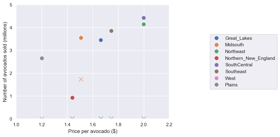
The circles represent sales quantity, and the cross markers represent the wasted quantity.
Notice how the ‘Wasted’ column reveals critical inefficiencies, particularly in the Midsouth region, where 1.73 units are lost despite accurate demand predictions. This suggests our allocation strategy may be overly rigid. What would happen if we ran a sensitivity analysis on the price-allocation relationship? A 10% price adjustment in high-waste regions could potentially recover more value than optimizing other variables. The data begs the question: where exactly should we relax constraints to minimize waste without compromising demand fulfillment?
More than that, these results reveal a clear tension between our model’s allocations and actual sales, particularly in the Midsouth, where we’re over-allocating by 1.73 units despite accurate demand predictions. This suggests our current constraints may be too rigid. Could we test:
- How sensitive is total waste to the 2.0 price ceiling in Northeast/SouthCentral/West?
- What happens if we make the Midsouth’s max_delivery constraint (currently 6.17) a decision variable instead of a fixed parameter?
- Would introducing a non-linear penalty for waste in the objective function change the allocation balance?
The model gives us the power to explore these scenarios systematically—should we run these sensitivity tests next?
OK, let’s go a bit further.
Optimization-Driven ML Pipelines: Where Prediction Meets Decision-Making
Training a single model in isolation is like building a car with only an engine—it might run, but it won’t perform optimally in real-world conditions. Machine learning pipelines, on the other hand, are the end-to-end assembly line that transforms raw data into robust predictions, ensuring efficiency, scalability, and reliability.
Machine learning pipelines outperform single-model approaches by automating the entire workflow from raw data to predictions, ensuring consistency and eliminating manual errors. Unlike standalone models that struggle with dirty data, pipelines integrate preprocessing, feature engineering, and model training into a unified system. They enable scalable deployments, simplify experimentation, and prevent data leakage through built-in cross-validation.

Pipelines also future-proof systems by modularizing components, allowing easy upgrades to preprocessing steps or models without disrupting production. Tools like Scikit-Learn’s Pipeline or TFX turn fragile prototypes into robust solutions. Single models might suffice for quick experiments, but pipelines are essential for real-world performance, maintainability, and business impact. The choice is clear: pipelines industrialize machine learning, while single models remain academic exercises.
Besides that, the convergence of machine learning and mathematical optimization represents a transformative leap in decision-making capabilities. Thanks to Gurobi, there is an open-source Python project that enables this powerful integration by allowing trained predictive models to become active components within optimization frameworks. This creates a seamless pipeline where data-driven predictions directly inform optimal decisions. The project is called Gurobi Machine Learning.
At its core, this integration works through a sophisticated two-stage process. First, machine learning models - whether developed in scikit-learn, TensorFlow/Keras, or PyTorch - are trained to understand complex relationships in operational data, such as how pricing affects demand or how production variables influence quality. These models capture the nuanced, often non-linear patterns that traditional optimization constraints struggle to represent.
The true innovation comes in the second stage, where these trained models are embedded directly as constraints within Gurobi’s optimization environment. This transforms predictive insights into prescriptive solutions. Where conventional approaches might treat machine learning predictions as static inputs, the Gurobi integration maintains the dynamic relationship between decision variables and predicted outcomes throughout the optimization process.
In that sense, we can establish the following goals:
- Simplify the process of importing a trained machine learning model built with a Popular ML package into an optimization model.
- Improve algorithmic performance to enable the optimization model to explore a sizable space of solutions that satisfy the variable relationships captured in the ML model.
Putting It All Together: A Clean Machine Learning Pipeline
Since we’re dealing with parametric models, we prepare the data using OneHotEncoder and make_column_transformer. We want to transform the region feature using the encoder while we apply scaling to the other features.
feat_transform = make_column_transformer(
    (OneHotEncoder(drop="first"), ["region"]),
    (StandardScaler(), ["price"]),
    ("passthrough", ["peak"]),
    verbose_feature_names_out=False,
    remainder="drop",
)


regions = [
    "Great_Lakes",
    "Midsouth",
    "Northeast",
    "Northern_New_England",
    "SouthCentral",
    "Southeast",
    "West",
    "Plains",
]
df = avocado[avocado.region.isin(regions)]

X = df[["region", "price", "peak"]]
y = df["units_sold"]
At this point, taking advantage of Gurobi ML tools is a mandatory step.
So why not compare models in order to get the model that best captures the relationship between variables ?
Let’s do this.
regressions = {
    "Linear Regression": {"regressor": LinearRegression()},
    "MLP Regression":    {"regressor": MLPRegressor([8] * 2, max_iter=1000, **args)},
    "Decision Tree":     {"regressor": DecisionTreeRegressor(max_leaf_nodes=50, **args)},
    "Random Forest":     {"regressor": RandomForestRegressor(n_estimators=10, max_leaf_nodes=100, **args)},
    "Gradient Boosting": {"regressor": GradientBoostingRegressor(n_estimators=20, **args)},
    "XGB Regressor":     {"regressor": XGBRegressor(n_estimators=20, **args)},
}

# Add polynomial features for linear regression and MLP

regressions_poly = {}
for regression in ["Linear Regression", "MLP Regression"]:
    data = {"regressor": (PolynomialFeatures(), clone(regressions[regression]["regressor"]))}
    regressions_poly[f"{regression} polynomial feats"] = data

# Merge the dictionary of polynomial features
regressions |= regressions_poly
Now we have a bunch of regression models, let’s train.
for regression, data in regressions.items():

    regressor = data["regressor"]

    if isinstance(regressor, tuple):
        lin_reg = make_pipeline(feat_transform, *regressor)
    else:
        lin_reg = make_pipeline(feat_transform, regressor)

    train_start = time()
    lin_reg.fit(X_train, y_train)
    data[("Learning", "time")] = time() - train_start
    data["pipeline"] = lin_reg

    # Get R^2 from test data
    y_pred   = lin_reg.predict(X_test)
    r2_test  = r2_score(y_test, y_pred)
    y_pred   = lin_reg.predict(X_train)
    r2_train = r2_score(y_train, y_pred)

    data[("Learning", "R2 test")] = r2_test
    data[("Learning", "R2 train")] = r2_train

    print(f"{regression:<18} R^2 value in the test set is {r2_test:.3f} training {r2_train:.3f}")
After that we can prepare the data for the optimization model.
| Region | Transport Cost | Min Delivery | Max Delivery |
|---|---|---|---|
| Great_Lakes | 0.3 | 2.063574 | 7.094765 |
| Midsouth | 0.1 | 1.845443 | 6.168572 |
| Northeast | 0.4 | 2.364424 | 8.836406 |
| Northern_New_England | 0.5 | 0.219690 | 0.917984 |
| SouthCentral | 0.3 | 3.687130 | 10.323175 |
| Southeast | 0.2 | 2.197764 | 7.810475 |
| West | 0.2 | 3.260102 | 11.274749 |
| Plains | 0.2 | 1.058938 | 3.575490 |
m = gp.Model("Avocado_Price_Allocation")
p = gppd.add_vars(m, data, name="price", lb=a_min, ub=a_max)
d = gppd.add_vars(m, data, name="demand") # Add variables for the regression
w = m.addVar(name="w") # excess wasteage
m.update()
m.setObjective((p * d).sum() - c_waste * w - (c_transport * d).sum())
m.ModelSense = GRB.MAXIMIZE
m.addConstr(d.sum() + w == B)
m.update()
for regression, data in regressions.items():
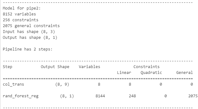
pred_constr = add_predictor_constr(m, data["pipeline"], feats, d, epsilon=1e-5)
pred_constr.print_stats()
data[("Optimization", "#constrs")] = m.NumConstrs + m.NumQConstrs + m.NumGenConstrs
data[("Optimization", "#vars")] = m.NumVars
m.Params.NonConvex = 2
m.Params.OutputFlag = 0
try:
start = time()
m.optimize()
data[("Optimization", "time")] = time() - start
data[("Optimization", "value")] = m.ObjVal
data[("Optimization", "viol")] = m.MaxVio
data[("Optimization", "error")] = pred_constr.get_error().max()
except gp.GurobiError:
data[("Optimization", "value")] = float("nan")
data[("Optimization", "viol")] = float("nan")
data[("Optimization", "error")] = float("nan")
break
pass
pred_constr.remove()Some points here:
- Function add_predictor_constr creates the formulation for the regression model and returns a modeling object.
- If the input of add_predictor_constr has several rows, introduce one corresponding model for each row.
- Models for logistic regression use a piecewise linear approximation and can have modeling error (controlled by parameters).
- Models for decision tree can also introduce small errors at threshold values of node splitting (can be controlled).
The following output reports a Random Forest regressor model.
Results
| Model | Learning Time | R² Test | R² Train | Opt. Constrs | Opt. Vars | Opt. Time | Opt. Value | Violation | Error |
|---|---|---|---|---|---|---|---|---|---|
| Linear Regression | 0.097 | 0.868 | 0.882 | 17 | 89 | 0.180 | 36.715 | 0.0 | 0.0 |
| MLP Regression | 2.018 | 0.883 | 0.894 | 273 | 345 | 5.581 | 39.001 | 0.0 | 0.0 |
| Decision Tree | 0.023 | 0.882 | 0.906 | 140 | 489 | 0.024 | 47.428 | 0.0 | 0.0 |
| Random Forest | 0.081 | 0.874 | 0.924 | 2332 | 8169 | 1.661 | 45.581 | 0.0 | 0.0 |
| Gradient Boosting | 0.110 | 0.802 | 0.829 | 972 | 1529 | 0.036 | 51.671 | 0.0 | 0.0 |
| XGB Regressor | 0.439 | 0.887 | 0.921 | 3219 | 5873 | 4.046 | 41.759 | 0.0 | 0.0 |
| Linear Regression (poly feats) | 0.048 | 0.884 | 0.894 | 457 | 529 | 0.026 | 42.101 | 0.0 | 0.0 |
| MLP Regression (poly feats) | 1.743 | 0.887 | 0.897 | 713 | 785 | 9.922 | 44.743 | 0.0 | 0.0 |
The presented data compares the performance of various regression models across multiple metrics, including learning time, R² scores on test and training sets, optimization constraints, variables, time, value, and violations. Linear Regression demonstrates a balanced performance with a learning time of 0.097 seconds, achieving an R² test score of 0.868 and an R² train score of 0.882. It also exhibits efficient optimization, requiring only 0.180 seconds with 17 constraints and 89 variables, yielding an optimal value of 36.715 without violations or errors.
The MLP Regression model shows improved predictive accuracy with R² scores of 0.883 (test) and 0.894 (train) but incurs higher computational costs, taking 2.018 seconds for learning and 5.581 seconds for optimization, involving 273 constraints and 345 variables. The Decision Tree model achieves competitive R² scores (0.882 test, 0.906 train) with minimal learning time (0.023 seconds) and optimization time (0.024 seconds), though its optimal value (47.428) is higher than that of Linear Regression.
Random Forest and Gradient Boosting models exhibit strong training performance (R² train scores of 0.924 and 0.829, respectively) but differ in generalization, with Random Forest maintaining a higher test R² (0.874) compared to Gradient Boosting (0.802). The XGB Regressor stands out with the highest test R² (0.887) and a strong training R² (0.921), albeit with substantial optimization complexity (3219 constraints, 5873 variables) and longer optimization time (4.046 seconds).
Incorporating polynomial features, Linear Regression and MLP Regression show marginal improvements in R² scores (0.884 and 0.887 for test, respectively), but the MLP model incurs a significant optimization time increase (9.922 seconds) due to higher constraint and variable counts (713 and 785, respectively). Overall, the XGB Regressor and polynomial-enhanced models demonstrate superior predictive accuracy, while Linear Regression remains the most computationally efficient choice for scenarios requiring rapid training and optimization.
Conclusions
In a very practical way, it’s possible to understand the benefits this tool offers. Despite some limitations, such as constraints on supported ML models, other questions arise:
- How can we ensure that optimization doesn’t misuse the results of the predictor?
- How to decide which prediction model to use?
- How would this make areas like ML less of a “black box”?
Even so, this represents more than just an incremental improvement in analytics—it creates a new paradigm for data-driven operations. The combination preserves the strengths of both disciplines: machine learning’s ability to extract insights from complex data and mathematical optimization’s capacity to find rigorous, optimal solutions. The result is a decision-making infrastructure that adapts as relationships change, learns as new data becomes available, and always seeks the best possible outcome given current understanding.
Alternatively, considering a research methodology, we can easily use this tool to establish experiment benchmarks. In our experiment above, we could have easily reversed the order and generated multiple models simultaneously, ultimately selecting and thoroughly evaluating the best one, conducting sensitivity analyses, or more specific experiments.
As I mentioned at the beginning, this tool opens up a range of opportunities—my main insight is to apply it to the financial market. I hope this content has been useful, inspiring, and helpful to you in some way.
Final Thoughts
If you’ve read this post so far, thank you very much, I hope this material has been useful and makes sense to you, and if any other topic related or not to the content of this post interests you, or has left you in doubt, put it in the comments and I will be very happy to bring the content more clearly in a new post.
Remembering that any feedback, whether positive or negative, just get in touch via my twiter, linkedin, Github or in the comments below. Thanks.
References
[1] Using Trained Machine Learning Predictors in Gurobi
[3] SAn Integrated Predictive and Prescriptive Modeling Framework
[4] OptiCL: Mixed-integer optimization with constraint learning
[5] reluMIP: Open Source Tool for MILP Optimization of ReLU Neural Network