


Over the past fifty years, researchers in empirical finance have explored the statistical properties of market indexes, commodities, and stock prices using data from a variety of markets and instruments. However, in the last ten years, the availability of large data sets of high-frequency price series and the use of computationally intensive methods for property analysis have opened up new avenues for research and have helped to solidify the use of data-based approaches in financial modeling.
Some long-standing disagreements about the nature of the data have been resolved as a result of the analysis of these new data sets, but it has also brought forth new difficulties. The ability to synthesize and meaningfully represent the qualities and information contained in this massive amount of data is not the least of them. Independent investigations have identified a collection of characteristics that are shared across numerous instruments, markets, and historical periods and have been categorized as “stylized facts”.
Empirical Approach
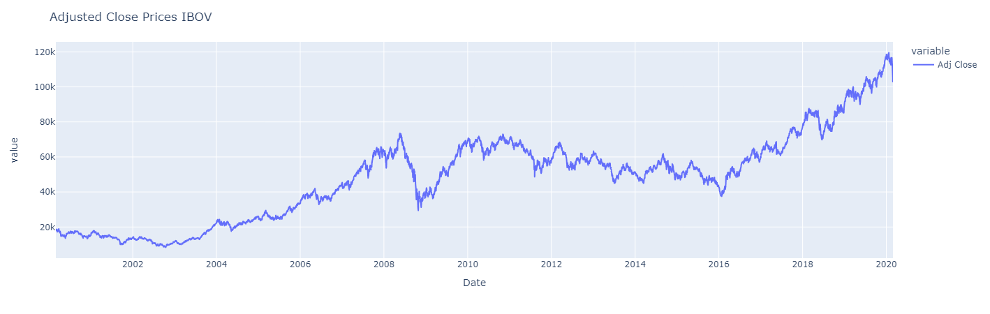
Let’s examine the daily adjusted closing values of the Bovespa index(IBOV) and the daily closing prices of Petrobras(PETR4) - Data includes values from January, 2000 to March, 2020.
The Bovespa Index (Ibovespa, or IBOV) is the most important indicator of the average performance of stocks traded on the São Paulo Stock Exchange. The index is composed of a theoretical portfolio with stocks that represented 80% of the traded volume in the previous 12 months and were present on at least 80% of the days when there was trading activity. The number of index components is not fixed, ranging between 60-80 assets.
Stationary time series is a time series whose statistical properties do not change over time.Stationarity is a desirable property of time series for statistical analysis. Prices of stocks are often not stationary as they exhibit a trend or seasonal component. To overcome this issue, we have considered log returns for statistical analysis instead of stock prices. Log returns are defined as follows.
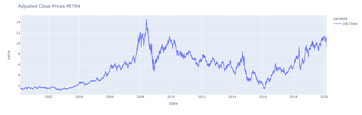
First of all let’s plot the adjusted closed prices series with periods of appreciation and devaluation.
Let’s visualize three distinct periods of returns from the Ibovespa Index.
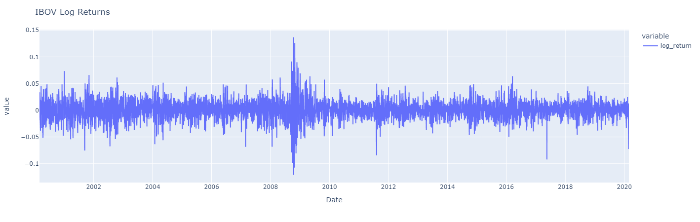
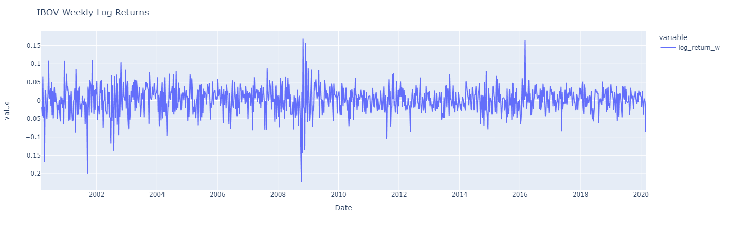
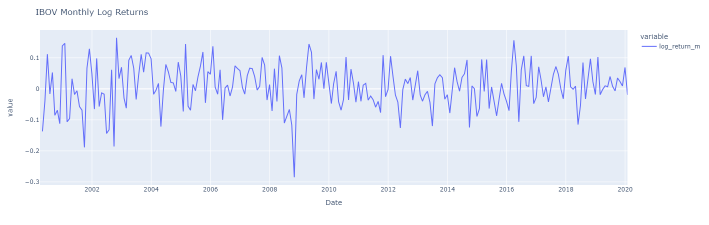
The three charts are similar, but monthly log returns are a smoother version of daily log returns, which display greater fluctuations. Besides, it can be observed that the high volatility during the periods from 2008 to 2020 is more pronounced in the daily chart. In contrast to prices series, returns fluctuate around a constant level, close to zero. Additionally, high fluctuations tend to “cluster,” reflecting more volatile market periods.
These characteristics are also evident in the data of PETR4, which follows.
Let’s visualize the same three distinct periods of returns from the PETR4.
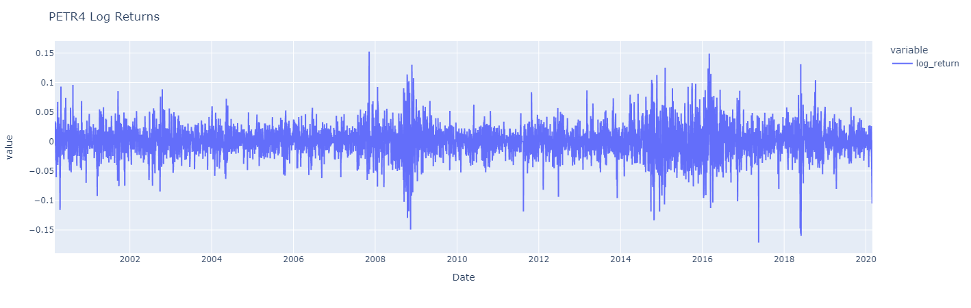
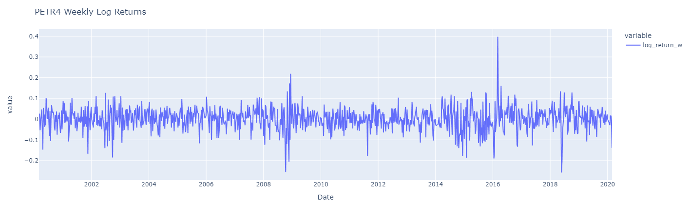
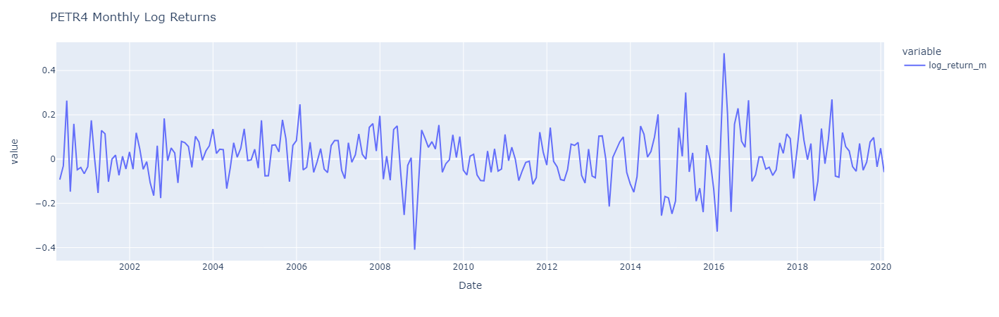
Again the three charts are similar, but monthly log returns are a smoother version of daily log returns, which display greater fluctuations with moments with higher volatility and moments with low volatily. However, it’s worth noting that its returns typically fluctuate around a constant level, suggesting at least a constant average over time.
Let’s go ahead and evaluate the distribution of these returns.
Are stock returns normally distributed ?
The distribution of returns
In statistics, a Q–Q plot (quantile-quantile plot) is a probability plot, which is a graphical method for comparing two probability distributions by plotting their quantiles against each other. If the two distributions being compared are similar, the points in the Q–Q plot will approximately lie on the identity line \(y = x\).
To continue with our analysis, we will evaluate the distributions of IBOV and PETR4 returns and understand how close these distributions are to a normal distribution.
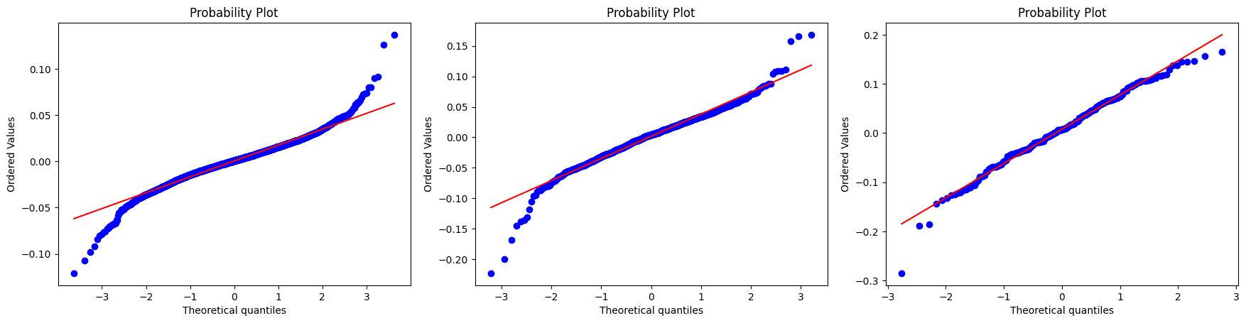
From image above we note that the tails of the return distributions are heavier than those of the normal distribution. Let’s observe now histograms of the daily, weekly, and monthly log-returns of the IBOV index, with normal density functions having the same mean and variance.
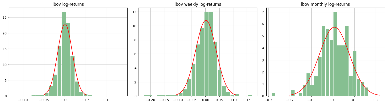
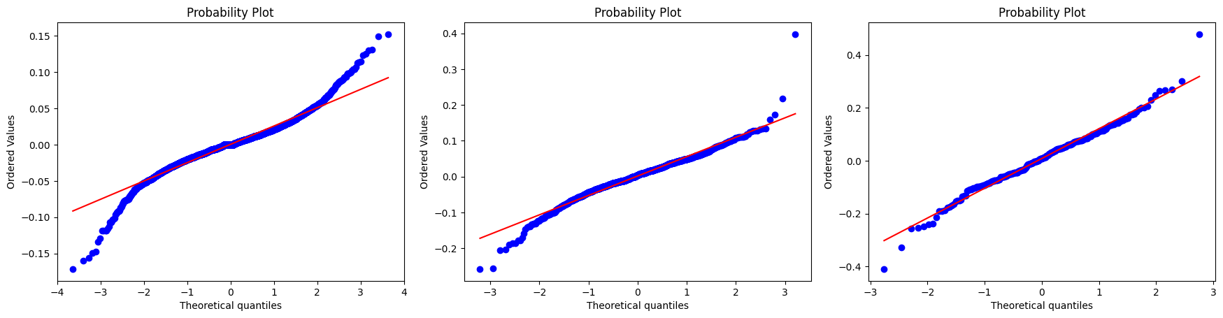
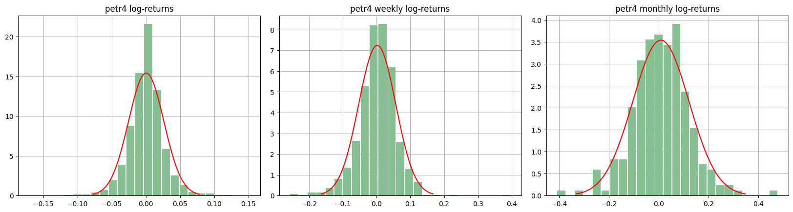
There are some concepts to be observed here. Note that as the range of returns increases in the distributions, from one day to one week and one month, the tails of the distribution become lighter. Particularly the distribution of monthly returns, which is relatively close to the normal distribution. The distributions are somewhat asymmetric due to the presence of high negative/positive returns. Not surprisingly, similar patterns can be observed in the log-return data of PETR4; see below.
Furthermore, it is possible to observe that the right tail of the distributions present small and very extreme returns, something very different from what a normal distribution would suggest. This phenomenon is observed more frequently in the distribution of daily returns, somewhat less in the distribution of weekly returns and even less in the distribution of monthly returns.
Autocorrelation function of the price changes
In time series analysis, autocorrelation refers to any statistical, whether causal or not, relationship between past and present values of a random variable.
But what does this mean? In technical terms, autocorrelation measures the correlation between the values of a data series and its own lagged values over time (the value of the observation at index t against the indices \(t-1, t-2, t-3\), and so on). In simpler terms, autocorrelation assesses the relationship between consecutive observations in a time series.
The ACF \(\hat{\rho}_{k}\) is defined at an shift \(k\) where given a series \(r_{1}, . . . , r_{T}\) the autocorrelation function is defined as \(\hat{\rho}_{k} = \hat{\gamma}_{k}/\hat{\gamma}_{0}\), onde
\begin{equation} \hat{\gamma_{k}} = \frac{1}{T}\sum_{t=1}^{T-k}(r_{t}-\overline r)(r_{t+k}-\overline r), \ \ \overline r=\frac{1}{T}\sum_{t=1}^{T}r_{t} \end{equation}
where \(\hat{\gamma}_{k}\) is the series covariance in the shift \(k\).
when plotting the autocorrelation function of the ibov log returns we have
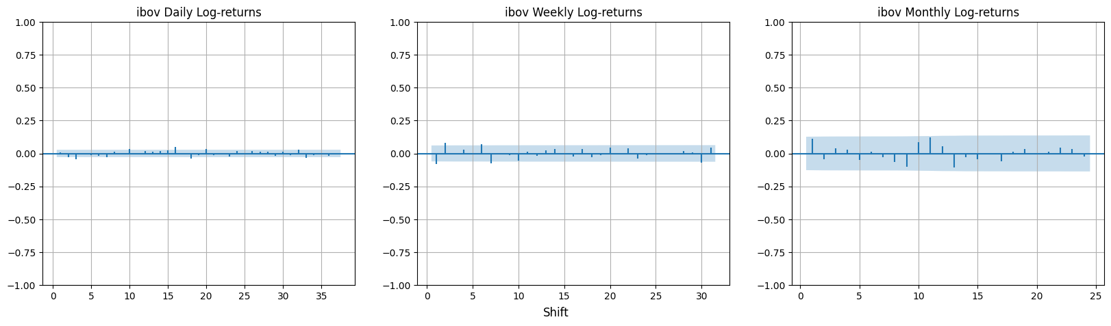
The two striped horizontal lines, which are defined as \(±1.96/\sqrt{T}\), are the limits of the 95% confidence interval for \(\rho_{k}\) if the actual value of \(\rho_{k} = 0\). Therefore \(\rho_{k}\) would be seen as not significantly different from zero if the estimate \(\hat{\rho}_{k}\) lies between these lines.
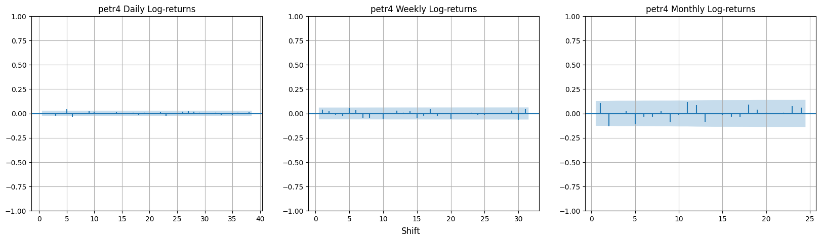
It is possible to observe that all daily, weekly and monthly log-returns do not exhibit significant autocorrelation. This corroborates the hypothesis that returns on a financial asset are uncorrelated over time or that there is no significant autocorrelation. This means that if such a correlation existed, it would be possible to predict the direction of the market based on historical data, in other words, it would be possible to create a strategy that predicts correctly and provides guaranteed profits. As a consequence of this, any investor would use this strategy by applying pressure on the purchase movement and causing the purchase price to be higher than the sale price, increasing the price and thus eliminating all possible gains. A possible exception to this rule would be very short time intervals, which would be the time needed for the market to react to new information. The same occurs to PETR4 log-returns.
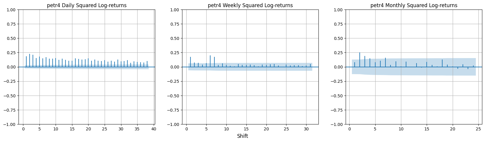
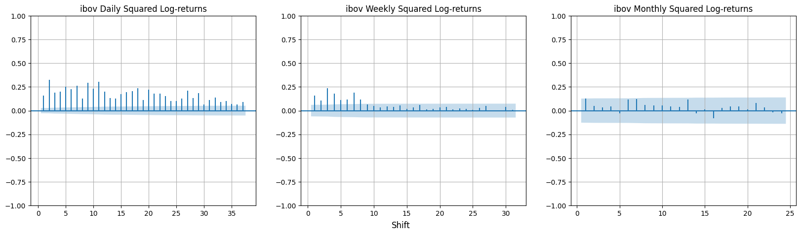
In the autocorrelation functions for squared log-returns and absolute value, \(r_{t}\) is replaced by \(r^2_{t}\) and \(\vert r_{t} \vert\). There are small but significant autocorrelations in \(r^2_{t}\) and even larger ones in \(\vert r_{t} \vert\). The more pronounced and persistent autocorrelations are found in daily data compared to weekly or monthly data. Empirical evidence suggests linear independence among returns, but with some non-linear self-dependence.
The results seen so far, derived from two sets of real data, align with the so-called Stylized Facts. Stylized facts are theoretical approximations of phenomena observed empirically. These “phenomena” are observed in different types of assets, including stocks, portfolios, commodities, and currencies.
What is a Stylized Fact?
According to an examination of most financial newspapers and journals, many market analysts have and continue to take an event-based approach, in which they attempt to “explain” or rationalize a given market movement by relating it to an economic or political event or announcement [1]. From this perspective, it is easy to conclude that, because different assets are not always influenced by the same events or information sets, price series obtained from different assets and, by extension, markets will exhibit distinct features.
But, on the other hand, is it wise to conclude corn prices behave similarly to IBM shares or the Dollar/Yen exchange rate?
The fact is that empirical studies on financial time series show that when examined statistically, a series of assets, which present purely random variations, share some non-trivial statistical characteristics. Stylized empirical facts refer to characteristics of asset series that prevail across a wide range of instruments, markets, and historical periods.
Stylized facts are obtained by combining qualities observed in many marketplaces and instruments. Obviously, doing so increases generality while decreasing the precision of statements about asset returns specifically. Indeed, stylized facts are typically expressed in terms of qualitative asset return characteristics and may be insufficient to distinguish between different parametric models.
Stylized Empirical Facts
Let me introduce a set of stylized statistical facts which are common to a wide set of financial assets.
Univariate Distributional Stylized Empirical Facts
Gain/Loss Asymmetry
Huge drawdowns in stock prices and index values, but not equally large upward movements. The distribution of returns normally has negative skewness. In other words, when considering any distribution, we would like the tail on the left and right sides to be symmetrical. However, in the real world return distributions have asymmetric tails and this is explained because in general periods of decline are generally more abrupt than periods of recovery. Besides that, investors tend to react more strongly to negative news than to positive news.
Leverage effect
Most indicators of an asset’s volatility are negatively linked to its returns, meaning periods of high volatility usually imply periods of decline.The term leverage derives precisely from the fact that as prices fall, companies become more leveraged (the ratio between debt and equity grows) and more risky, and therefore their prices become more volatile. Therefore, the volatility caused by drops in prices is typically greater than the appreciations caused by drops in volatility.
The majority of asset volatility metrics show a negative correlation with the asset’s returns [2]. Variance of returns over a certain time period is one metric used to quantify a stock’s volatility. Since, mean returns for many of the stocks are zero, we consider squared returns as a measure of volatility. For random variables \(X\) and \(Y\), we define correlation coefficient as follows:
\begin{equation} \rho = \frac{cov(X,Y)}{\sigma_{X}\sigma_{Y}} \end{equation}
Where:
\(cov(X,Y) = E(XY) - E(X)E(Y)\), \(\sigma^2_{X} = Var(X)\), \(\sigma^2_{Y} = Var(Y)\)
We calculate the correlation coefficient between log returns and squared returns of the same stock(PETR4 or IBOV). A positive correlation coefficient signifies the positive association of two variables whereas a negative correlation coefficient signifies the negative association of two variables. According to the stylized facts, the correlation coefficient between log returns and squared returns is expected to be negative, as we have shown before.
Disclaimer: This absence of autocorrelation in time does not necessarily mean independence: simple non-linear functions, such as absolute value, exhibit positive and persistent self-correction, indicating long-term memory properties.
Autocorrelations in non-linear functions become weaker and less persistent when the interval of returns is changed from a day to a week or a month.
Aggregational Gaussianity
The distribution of results resembles a normal distribution as the time scale \(\Delta t\) over which they are computed grows. Specifically, the distribution’s form varies across different time scales. In other words, when the time horizon increases, the distribution of returns tend to more closely approximate the normal distribution. We can observe this in the Q-Q plot generated for the IBOV and PETR4 distributions.
Kolmogorov-Smirnov Test, Shapiro-Wilke Test and Jarque-Bera Test were used to test the normality of daily, weekly, monthly returns.p-values were recorded for each test conducted. According to the stylized fact, p-value is expected to increase as we move from daily to quarterly returns for same stock.
Heavy tails
Return series generally exhibit heavier tails than the tail of a normal distribution. The (unconditional) distribution of returns appears to have a power-law or Pareto-like tail, with a tail index that is finite, more than two but less than five for the majority of data sets investigated. This excludes stable rules with infinite variance, as well as the normal distribution. However, the exact shape of the tails is difficult to identify. This phenomenon can be visually observed in the histograms and Q-Q plots of the IBOV and PETR4 series.
However, one way to quantify the weight of the tail as well as the size of the deviation from normality is using kurtosis (a.k.a normalized statistical fourth moment). By default, the kurtosis of a theoretical normal distribution has its value set at \(3\). If the kurtosis of a given distribution is greater than \(3\), the tendency is for such a distribution to have a heavier tail than the normal one, which is normally the case for distributions of financial returns.
Return distributions tend to be Non-Gaussian, with a peak sharp and heavy tails, with these properties more pronounced for intraday data, given that distributions with more frequent data tend to have even heavier tails
Multivariate Stylized Empirical Facts
Volume-Volatility Correlation
Trading volume is correlated with all measures of volatility. The correlation coefficient between log returns and trading volume has been calculated for every stock under consideration. According to the stylized fact,the correlation coefficient between log returns and trading volume is expected to be positive.
Risk-Return Tradeoff
Risk incurred in investment in a particular financial instrument and returns of that financial instrument are correlated. Volatility of a stock has been considered as measure of risk. Here, the measure of volatility used is standard deviation of returns of a particular stock over full period of consideration. The correlation coefficient between mean return (Calculated over full period of consideration) and standard deviation of returns of stocks listed on a particular stock market has been calculated. According to the stylized fact, this correlation coefficient is expected to be positive for every market considered.
Time series Related Stylized Empirical facts
Absence of Autocorrelations
The Autocorrelation measures the similarity between a time series and its version with lag at different time intervals. (Linear) autocorrelations of asset returns are frequently minimal, particularly on very brief intraday time scales (about 20 minutes), where microstructure effects come into play.
Returns in liquid markets do not exhibit self-correction when significant. When calculating the self-correction of a series with itself 1 shift to the right, it is possible to observe that the series presents very small and insignificant values. This particular fact is often cited as support for the efficient market hypothesis.
If there were significant autocorrelation, it would be possible to predict the direction of the market based on historical data. In other words, it would be possible to create a strategy that predicts the market direction accurately and provides guaranteed profits (Arbitrage). This would cause the strength of the buying moves to increase which in turn would eliminate all possible gains. A possible exception to this rule would be very short time intervals, which represent the time it takes the market to react to new information.
Long-term Dependence:
The absence of autocorrelations provided empirical support for models based on “Random Walks” where returns are considered independent random variables. Therefore random walks assume that the random variables that are governed by these stochastic processes (Random Walks) are independent of each other. That is, the value of today’s return is completely dependent on yesterday’s return.
However, this is not necessarily true because as we have seen, there is actually some type of non-linear correlation dependence. This becomes clear when we present the ACF of absolute log returns and squared log returns - especially log absolute returns. This type of non-linear dependence is present in return series and it is possible to exploit it in a beneficial way if we wish to create some strategy. One thing that can also be observed is that there is a downward trend shown by the ACF of the two series of assets until it eventually reaches zero. This statistical property is called Ergodicity
Ergodicity: In a stationary stochastic process in covariance, we make no assumptions about the intensity of dependence between the variables in the sequence.
consider:
\begin{equation} \rho_{1} = corr(Y_{t}, Y_{t-1}) = \rho_{100} = corr(Y_{t}, Y_{t-100}) = 0.5 \end{equation}
However, in many contexts it is reasonable to assume that the intensity of dependence decreases with distance in time. That is, \(\rho_{1} > \rho_{2} > \rho_{3} > ...\) and eventually \(\rho_{j} = 0\) for a sufficiently large \(j\).
Volatility Clustering
Different measures of volatility show a positive autocorrelation across several days, indicating that high-volatility occurrences tend to cluster in time. In other words, Non-linear dependence is directly related to the well-known phenomenon of volatility clustering: large changes in the price of an asset are usually followed by other large variations. Furthermore, it is common to observe this phenomenon in almost all markets on the planet.
For example: it is possible to observe that the standard deviations of IBOV daily returns in 2007 were \(1.7\%\), \(2.0\%\) in the first half of 2008 and \(1.9\%\) in 2009. In the second half of 2008(Subprime risis) it was \(4.1\%\) due to the several days of crisis and high volatility.
Intermittency
results show a significant degree of fluctuation across all time scales. This is measured by the occurrence of irregular bursts in time series from a wide range of volatility estimators. Intermittency can be characterized by high kurtosis. Kurtosis was computed for the return series and also for residual series obtained after fitting a GARCH model(to eliminate the time series effect from the data).
Kurtosis for a random variable \(X\) is defined as
\begin{equation} K = \frac{E(X - \mu)^4}{\sigma^4} \end{equation}
Where \(\mu = E(X)\) and \(\sigma^2 = Var(X)\)
As we mentioned before, The value of kurtosis for normal distribution is \(3\). The one sided test to check if kurtosis is \(3\) against the alternative hypothesis that kurtosis is greter than was carreied out using the test statistic \(\frac{\sqrt(n)(K-3)}{\sqrt(24)}\) which follows asymptotic normal distribution. p-values were computed in each case. Acoording to the stylized fact, the p-values are expected to be small i.e the null hypothesis that kurosis is 3 is expected to get rejected.
Conclusion
In the previous sections, we presented statistical phenomena about asset returns that are consistent across multiple assets and markets. These features are based on qualitative hypotheses rather than parametric assumptions about the return process. These requirements are necessary for a stochastic process to accurately recreate the statistical features of returns. Current models struggle to recreate all statistical traits simultaneously, highlighting their limitations.
Finally, we should mention a few difficulties that we haven’t covered here. One significant question is whether a stylized empirical truth has economic relevance. In other words, can these empirical findings be utilized to corroborate or refute specific modeling methodologies used in economic theory? Another concern is if these empirical findings are valuable for practitioners. For example, does the occurrence of volatility clustering suggest anything useful for volatility forecasting? Can this lead to a more effective risk measurement and management approach? Can one use these correlations to develop a volatility trading strategy? Or, how can one include a measure of irregularity, such as the singularity spectrum or the extremal index of returns, into a risk measure for portfolios? We will leave these questions for future research.
Here at Turing Quant we try to take all these factors into consideration when we build our strategies and try to keep our portfolio optimized aiming for the best gains. It’s always a good time to take a stand. Do not let this chance go by.
Final Thoughts
If you’ve read this post so far, thank you very much, I hope this material has been useful and makes sense to you, and if any other topic related or not to the content of this post interests you, or has left you in doubt, put it in the comments and I will be very happy to bring the content more clearly in a new post.
Remembering that any feedback, whether positive or negative, just get in touch via my twiter, linkedin, Github or in the comments below. Thanks.