


Quadratic Programming (QP) models, such as the Markowitz model, are now relatively simple to answer due to technological and algorithmic advancements. Nonetheless, Linear Programming (LP) models remain significantly more appealing from a computational standpoint for a variety of reasons. The design and development of commercial software for solving LP models is more advanced than for QP models. As a result, various commercial LP solvers are available, and LP solvers are typically more trustworthy than QP solvers. On average, LP solvers can solve far bigger cases than QP solvers in a fraction of the time (on the order of seconds).
Is it possible to create linear models for portfolio optimization? How can we assess risk or safety to create a linear model?
A first observation is that, in order to ensure that a portfolio benefits from diversification, no risk or safety measure can be a linear function of the portfolio’s asset shares, through discretization of the return random variables or, equivalently, through the that is of the variables \(x_{j}, j = 1,...,n\). However, linear models can be obtained using the concept of scenarios.
Stochastic dominance and mean-risk models
Disclaimer: In the following section we will briefly introduce the concept of stochastic dominance. The Concept will be presented in a superficial way only for completeness of context since stochastic dominance is not the focus of the article.
The difficulty of choosing between investment opportunities or portfolios with uncertain returns is a special case of comparing uncertain outcomes. The latter is of vital interest to decision theory. Assuming basic rationality axioms, allowing an investor to organise all potentially risky possibilities in a continuous and consistent manner implies that investor behaviour can be modelled as being driven by a real-valued utility function used to compare outcomes. This is the “expected utility hypothesis.” In practice, however, it is nearly difficult to determine the exact utility function precisely. Nonetheless, one can identify utility function requirements or qualities based on preferences shared by all rational investors. For example, suppose the utility function is non-decreasing, which means that more is preferred over less (maximization). Such universal preferences define a partial order of risky outcomes, known as stochastic dominance. The stochastic dominance technique provides a theoretical framework, but not a straightforward computational recipe for determining the best portfolio. The portfolio optimization models presented here are based on the mean-risk or mean-safety approach, which quantifies the problem using only two criteria: the mean, which represents the expected outcome, and the risk or safety, which is a scalar measure of the variability of outcomes. It is critical to determine whether the models follow the partial order of risky outcomes. When they do, they are said to be consistent with the stochastic dominance. Unfortunately, for typical dispersion statistics as risk measures, like variance, the mean-risk approach consistency cannot be proved. A different, though related, concept, is that of coherent risk measure and is defined through properties of a risk measure that capture the preferences of a rational investor.
The challenge of optimal portfolio selection is similar to the problem of comparing probabilities provided by random variables with known distributions. The fundamental axioms of investor rationality, notably completeness, transitivity, independence, and continuity, necessitate the ability to define a utility function. This implies that a rational investor has a utility function \(u\) such that \(R_{x'}\) is prefered to \(R_{x''}\) if and only if \(\mathbb{E}(u(R_{x'}) \geq \mathbb{E}(u(R_{x''})))\). While it is impossible to determine a single investor’s utility function, it is crucial to identify criteria that all rational investors share. Stochastic Dominance (SD) is a family of partial orders that are closely related to expected utility theory, but do not require the explicit specification of a utility function. With stochastic dominance, random variables are ordered by point-wise comparison of functions built from their distribution.
The First-order Stochastic Dominance (FSD) relationship compares underachievement probability across all genuine targets \(\tau\).
\begin{equation} R_{x’}\succeq_{FSD} R_{x’’} \Leftrightarrow \mathbb{P}(R_{x’} \geq \tau) \geq \mathbb{P}(R_{x’’} \geq \tau) \ \ \ \forall \ \ \ \tau. \end{equation}
Thus, in FSD uncertain returns are compared by point-wise comparison of the right-continuous cumulative distribution function (cdf), \(F_{x}(\tau) = \mathbb{P}(R_{x} \leq \tau)\).
\begin{equation} R_{x’}\succeq_{FSD} R_{x’’} \Leftrightarrow F_{x’}(\tau) \leq F_{x’’}(\tau) \ \ \ \forall \ \ \ \tau. \end{equation}
We say that portfolio \(x'\) dominates \(x''\) under the FSD (and we write \(R_{x'} \succ_{FSD} R_{x''}\)) if \(R_{x'} \succeq_{FSD} R_{x''}\) and \(R_{x''} \nsucceq_{FSD} R_{x'}\). That means \(R_{x'} \succ_{FSD} R_{x''}\) if \(F_{x'}(\tau) \leq F_{x''}(\tau)\) for all \(\tau\), and there exists at least one \(\tau_{0}\) such that \(F_{x'}(\tau_{0}) \leq F_{x''}(\tau_{0})\)
A feasible portfolio \(x^0 \in \varrho\) is called FDS efficient if the is no \(x \in \varrho\) such that \(R_{x} \succ_{FSD} R_{x^0}\). The FSD relation represents general preferences that more is preferred to less.
The FSD, which assesses investor preferences, does not consider risk-taking behaviour. Investors are typically believed to be risk averse, in the sense that a certain yield of value \(\mathbb{E}(R_{x})\) is chosen over the hazardous return \(R_{x}\) for every \(R_{x}\) distribution. These generic risk-averse preferences establish the Second-order Stochastic Dominance (SSD). In portfolio optimization, the comparison of random variables representing returns is related to the problem of selecting hazardous alternatives from a given feasible set Q.
For example, in the most basic situation, the feasible set of random variables is defined as all convex combinations (weighted averages with non-negative weights totaling 1) of a given number of investment possibilities (assets). If \(R_{x'} \succeq R_{x''}\) then \(R_{x'}\) is preferred to \(R_{x''}\) within all risk-averse preference models where larger outcomes are preferred.
It is consequently critical that a model for portfolio optimization is consistent with the SSD relation. Note that due the SSD consistency implies FSD consistency, which applies to any models in which larger outcomes are chosen. If the risk measure \(\varrho(x)\) is SSD consistent in the sense that
\begin{equation} R_{x’}\succeq_{SSD} R_{x’’} \Rightarrow \varrho_{x’} \leq \varrho_{x’’} \end{equation}
The SSD consistency conditions fulfill only very specific shortfall risk measures like lower partial moments and particularly the mean below-target deviation that represents a single value of the second-order cumulative distribution function.
Typical dispersion-type risk measures when minimized may lead to choices inconsistent even with the FSD and, thus, not acceptable for any preference related to maximization of returns (better than less). As we’ll see in the next section.
Ok! A lot of concepts here. But keep in mind the following:
The main point of this section is to make clear for you that the SD relationship, compares the entirety of the portfolio distributions, thus preventing the potential problem of focusing on specific statistics while ignoring other statistical information. Besides, In the study of economic behavior, it is generally accepted that increasing and concave utility functions express the preference of risk-averse investors, which gives a theoretical justification for the importance of choosing SSD-efficient portfolios.
Risk and safety measures
Mean-risk models use two scalars to characterise and compare return distributions. One scalar is the expected value (mean); high expected returns are preferable. The other scalar represents the value of a “risk measure”. A risk measure assigns a number to each distribution, indicating its “riskiness”; low risk values are preferred. Preference for distributions is based on balancing risk and mean.
The risk metrics presented here are dispersion measures, which assess the degree of fluctuation in the portfolio rate of return around its expected value. This appears to be a reasonable method for measuring variability, but it has a downside. A portfolio with an extremely low return is efficient if the return can be achieved with confidence, i.e. if the dispersion is zero. Even when all possible rates of return are higher, such a portfolio is not dominated by any other riskier one. As we mentioned in the previous section, the Markowitz model is frequently criticized because its lack of consistent axiomatic models [1]. The Markowitz model is not consistent with the Second Degree Stochastic Dominance (SSD) since its efficient set may contain portfolios characterized by a small risk but also very low return [2]. Unfortunately, it is a common flaw of all Markowitz-type mean-risk models where risk is measured with some dispersion measures. This can be illustrated by two portfolios x’ and x’‘ (with rate of return given in percents).
Let’s consider the following example:
Example: Imagine we have two portfolios x’ and x’‘ with rate of return given in percents.
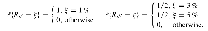
Both portfolios are efficient for any dispersion measure, with x’ having a lesser return than x’‘ but being risk-free. However, x’ with a guaranteed return of \(1\%\) is clearly worse than the risky portfolio x’‘, whose return may be \(3\%\) or \(5\%\). No logical investor would choose x’ to x’‘ because, regardless of the rate of return, portfolio x’‘ outperforms x’.
In order to overcome this weakness of the dispersion measures, the concept of safety measure, that is a measure that an investor aims at maximizing, was introduced. In that way we can define safety measure as measures the when embedded in an optimization model, are maximized instead of being minimized. We can also note that each risk measure \(\varrho(x)\) has a well defined safety measure \(\mu(x) - \varrho(x)\) and viceversa.
Although the risk measures are more ‘natural’, due to the consolidated familiarity with Markowitz model, the safety measures do not suffer of the drawback we observed for the dispersion measures.
A portfolio dominated in the mean-risk problem can be shown to be dominated also in the corresponding mean-safety problem. Indeed, if a portfolio x’ is dominated by a portfolio x’‘ in the mean-risk problem, then the return of the former is greater or equal the second one — \(\mu(x'') \geq \mu(x')\), and the risk of x’‘ is lower or equal to x’ — \(\varrho(x'') \geq \varrho(x')\). So, we can derive that:
\begin{equation} R_{x’}\succeq_{SSD} R_{x’’} \Rightarrow \varrho(x’’) - \mu(x’’) < \varrho(x’) - \mu(x’) \end{equation}
Thus, portfolio x’ is dominated by portfolio x’‘ also in the mean-safety problem. We can see that in the figure below
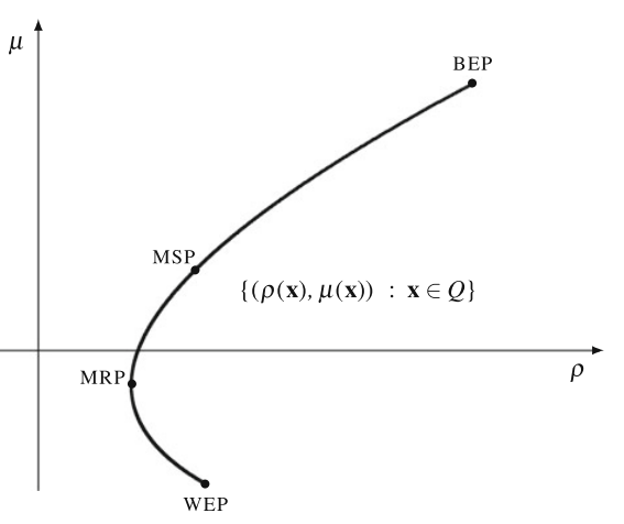
We know that the risk measure \(\varrho(x)\) is typically a convex function. Due to linearity of \(\mu(x)\) and convexity of \(\varrho(x)\), the portfolios \(x \in \varrho\) form a set with the convex boundary from the side od \(\mu\)-axis. This boundary illustrates a curve of the lowest risk portfolios, ranging from the best expectation portfolio (BEP) to the worst expectation portfolio (WEP). Minimum Risk Portfolio (MRP), defined as the solution of \(min \ \varrho(x)\) limites the curve to the mean-risk efficient frontier from BEP to MRP. Similarly, the Maximum Safety Portfolio (MSP), defined as the solution of max {\(\mu(x) - \varrho(x)\)}, distinguishes a part of the mean-risk efficient frontier, from BEP to MSP, which is also mean-safety efficient.
Thus we can derive that the minimum risk portfolio (MRP) is defined as a minimization solution, which on the efficient frontier above represents the minimum point that a portfolio must achieve considering the maximum acceptable risk (Maximum risk limit to be undertaken). On the other hand, the maximum safety portfolio (MSP) is defined as a maximization solution, which on the efficient frontier above represents the maximum point that a portfolio must achieve considering the maximum acceptable safe point (Maximum return limit without taking risks).
While the original Markowitz model forms a quadratic programming problem, many attempts have been made to linearize the portfolio optimization procedure. Certainly, to model advantages of a diversification, risk measures cannot be linear function of \(x\). Nevertheless, the risk measure can be LP computable in the case of discrete random variables, i.e., in the case of returns defined by their realizations under the specified scenarios. In the next section we will consider \(T\) scenarios with probabilities \(p_{t}\) (where \(t = 1,...,T\)). We will assume that for each random variable \(R{j}\) there is known its realization \(r_{jt}\) under the scenario \(t\). Typically, the realizations are derived from historical data treating \(T\) historical periods as equally probable scenarios (\(p_{t} = 1/t\)).
Scenario and LP Computability
Consider that \(R_{j}\) denotes the random variable indicating the rate of return of asset \(j, j = 1,...,n\), at the specified time. We now present the concept of scenario to address the uncertainty of the rates of return on assets at the target time. Informally, a scenario is a probable situation that could occur at the target time, in our case, the realisation of the asset’s rates of return at that time. Depending on what happens between the investment and target times, any of various eventualities could come true. The possibilities may be less or more probable to occur. More precisely, a scenario is a realisation of a multivariate random variable that represents the rates of return on all assets. Let’s consider the following scenarios:
| Asset | Scenario 1 (%) | Scenario 2 (%) | Scenario 3 (%) | Mean Return Rate (%) |
|---|---|---|---|---|
| 1 | \(r_{11}\) = 3.1 | \(r_{12}\) = -2.7 | \(r_{13}\) = 1.6 | \(\mu_{1}\) = 0.67 |
| 2 | \(r_{21}\) = 2.3 | \(r_{22}\) = -2.3 | \(r_{23}\) = 1.3 | \(\mu_{2}\) = 0.43 |
| 3 | \(r_{31}\) = 4.2 | \(r_{32}\) = -3.1 | \(r_{33}\) = -0.2 | \(\mu_{3}\) = 0.43 |
| 4 | \(r_{41}\) = 1.5 | \(r_{42}\) = -2.0 | \(r_{43}\) = -0.1 | \(\mu_{4}\) = -0.2 |
The table above illustrates an example with \(n = 4\) assets and \(T = 3\) situations. The scenario is optimistic, with all rates of return positive. Scenario 2 is negative, but scenario 3 is good for assets one and two but negative for assets three and four. The averages are calculated with the assumption that all situations are equally likely (\(p_{t} = 1/3, t = 1, 2, 3\)).
We now assume that, following a thorough preliminary investigation, \(T\) alternative scenarios are feasible at the target time. The chance that scenario \(t, t = 1,...,T\), will occur is given by \(p_{t}\). We assume that for each random variable \(R_{j}, j=1,...n\), its realization \(r_{jt}\) under scenatio \(t\) is known. The scenario \(t\) is defined by the set of returns for all assets \({r_{jt}, j = 1,...,n}\). The expected return of asset \(j, j = 1,...,n\), is computed using as \(\mu_{j} = \sum_{t=1}^{T} p_{t}r_{jt}\). The idea of scenario captures the correlation between asset rates of returns.
Identifying and estimating the rate of return (\(r_{jt}\)) for each asset under each scenario (\(t\)) is critical. To be statistically significant, the number of possibilities must be sufficiently large. Each portfolio x defines a corresponding random variable \(R_{x} = \sum_{j=1}^{n}R_{j}x_{j}\) that represents thr portfolio rate of return. The return \(y_{t}\) of a portfolio \(x\) in scenario \(t\) can be computed as:
\begin{equation} y_{t} = \sum_{j=1}^{n} r_{jt}x_{j} \end{equation}
The expected return of the portfolio \(\mu(x)\)can be calculated as a linear function of \(x\).
\begin{equation} \mu(x) = E[ R_{x}] = \sum_{t=1}^{T}p_{t}y_{t} = \sum_{t=1}^{T}p_{t} \Bigl( \sum_{j=1}^{n} r_{jt}x_{j} \Bigl) = \sum_{j=1}^{n} x_{j}\sum_{t=1}^{T} p_{t}r_{jt} = \sum_{j=1}^{n}\mu_{j}x_{j} \end{equation}
We defined a scenario as a realisation of the multivariate random variable that represents the asset’s return rates. The set of scenarios can be considered a discretization of the multivariate random variable. Returns are discretized when characterised by their realisations under specific circumstances, resulting in a set of values { \(r_{jt} : j = 1,...,n,t=1,...,T\) }. We will say that a risk or a safety measure is LP computable if the portfolio optimization model takes a linear form in the case of discretized returns.
Thus, A risk measure is linearly computable (LP-computable) if the portfolio optimization problem takes a linear form in the case of discretized returns. In other words, the risk portfolio optimization problem becomes linear with returns discretization. Note that, the variance isn’t LP-Computable, since its discrete form is a quadratic function.
Basic LP Computable Risk Measures
Disclaimer: In this section we’ll present the more usefull LP computable risk and safety measures. Despite that, these measures presented here aren’t the only available (i.e Below-target deviations, Omega Ratio Maximization).
The notion of risk is related to a possible failure of achieving some targets. It was formalized by [3] as the so-called safety-first strategies and later led to the concept of below-target risk measures [4] or shortfall criteria. In that way, the variance is a classical statistical metric that measures the dispersion of a random variable around its mean. There are, however, various methods for determining the dispersion of a random variable. The random variable that we are interested in is the portfolio return \(R_{x}\).
MAD - Mean Absolute Deviation
The MAD model introduced by [5] with a directly defined mean absolute deviation was not the first LP portfolio optimization model. Nevertheless, it has drawn a lot of attention resulting in much research and speeding up develop- ment of other LP models.
The Mean Absolute Deviation (MAD) is a dispersion measure that is defined as
\begin{equation} \delta(x) = \mathbb{E} = (|R_{x} - \mathbb{E}(R_{x})|) = \mathbb{E} (|\sum_{j=1}^{N}R_{j}w_{j} - \mathbb{E}(\sum_{j=1}^{N}R_{j}w_{j}) |) \end{equation}
The MAD model, like the Markowitz model, typically produced portfolios with the highest returns while also carrying the highest risk of underachievement. Certainly, the MAD metric can be applied to multi-period challenges in portfolio management. The MAD calculates the average of the absolute difference between a random variable and its expected value. The MAD takes absolute values into account rather than squared values when calculating variance, as a consequence it gives less importance to the extreme terms since we do not square. We demonstrate in the following that, when the returns are discretized, the MAD is LP calculable and can be wrtitten as:
\begin{equation} \delta(x) = \sum_{t=1}^{T}p_{t}(|\sum_{j=1}^{N}R_{jt}w_{j} - \sum_{j=1}^{N}\mu_{j}w_{j}|) \end{equation}
In that way, we have the difference between the portfolio return in scenario \(j\) and the expected portfolio return times the scenario probability. The portfolio optimization problem then becomes
\begin{equation} min \ \delta(x) = \sum_{t=1}^{T}p_{t}(|\sum_{j=1}^{N}r_{jt}w_{j} - \mu|) \end{equation}
\(\qquad \qquad \qquad \qquad \qquad \qquad\) s.t
\begin{equation} \sum_{j=1}^{N}\mu_{j}w_{j} = \mu \end{equation}
\begin{equation} \mu \geq \mu_{0} \end{equation}
\begin{equation} \sum_{j=1}^{N}w_{j} = 1 \end{equation}
\begin{equation} w \in Q \end{equation}
Where \(\mu_{0}\) is the lower bound on the portfolio expected return required by the investor, and \(Q\) indicates the system of constraints defining the set of viable portfolios. Note that the proposed form before is not linear in the variables \(w_{j}\) but can be transformed into a linear form. We now define the deviation in scenario \(t\) as \(d_{t}\), that is \(d_{t} = \sum_{j=1}^{N}\mu_{j}w_{j}\). Then the portfolio optmization problem is:
\begin{equation} min \ \delta(x) = \sum_{t=1}^{T}p_{t}d_{t} \end{equation}
\(\qquad \qquad \qquad \qquad \qquad \qquad\) s.t
\begin{equation} d_{t} = |y_{t} - \mu| \ \ \ \ \ \ \ \ t=1,…,T \end{equation}
\begin{equation} y_{t} = \sum_{j=1}^{N}R_{jt}w_{j} \ \ \ \ \ \ \ \ t=1,…,T \end{equation}
\begin{equation} \mu = \sum_{j=1}^{N}\mu_{j}w_{j} \end{equation}
\begin{equation} \mu \geq \mu_{0} \end{equation}
\begin{equation} \sum_{j=1}^{N}w_{j} = 1 \end{equation}
\begin{equation} w \in Q \end{equation}
Note that, despite the objective function following a linear form, now we have a non-linear constraint. Since \(\|y_{t} - \mu\| = max \{(y_{t} - \mu), (\mu - y_{t})\}\) the problem can be written in the following equivalent linear form:
\begin{equation} min \ \delta(x) = \sum_{t=1}^{T}p_{t}d_{t} \end{equation}
\(\qquad \qquad \qquad \qquad \qquad \qquad\) s.t
\begin{equation} d_{t} \geq y_{t} - \mu \ \ \ \ \ \ \ \ t=1,…,T \end{equation}
\begin{equation} d_{t} \geq \mu - y_{t} \ \ \ \ \ \ \ \ t=1,…,T \end{equation}
\begin{equation} y_{t} = \sum_{j=1}^{N}R_{jt}w_{j} \ \ \ \ \ \ \ \ t=1,…,T \end{equation}
\begin{equation} \mu = \sum_{j=1}^{N}\mu_{j}w_{j} \end{equation}
\begin{equation} \mu \geq \mu_{0} \end{equation}
\begin{equation} \sum_{j=1}^{N}w_{j} = 1 \end{equation}
\begin{equation} w \in Q \end{equation}
The equivalence comes from the fact that if \(y_{t} - \mu \geq 0\), constraints \(d_{t} \geq y_{t} - \mu\) and \(d_{t} \geq \mu - y_{t}\) are redundant, and is desired that both constraints should be true. In this case that constraints combined with minimization of \(\sum_{t=1}^{T}p_{t}d_{t}\) pushes the value of each \(d_{t}\) to the minimnum value allowed by the constraints, impose that \(d_{t} = y_{t} - \mu = \|y_{t} - \mu\|\). Thus we have now a fully linear model that minimizes MAD depite the indirectly way.
The MAD model was proposed by Konno (1991) as an alternative model to Markowitz. His main motivation was to avoid computational difficulties of the quadratic Markowitz problem. Konno showed that the optimal portfolios generated with MAD are quite similar to those of Markowitz. In fact, if they are normally distributed, the solutions are identical. Furthermore, the ease in solving the model allows you to solve larger instances and more realistic problems.
To summarize, the optimization model above is a linear programming model for portfolio optimization problems, where risk is evaluated through the MAD of the portfolio’s return. It is also worth mentioning that MAD model, unlike the Markowitz model, does not assume normality of returns since its input is a discretized joint distribution generated from the scenario matrix.
The MAD takes into account any deviations in the portfolio’s rate of return from its expected value, both below and above that value. However, one may reasonably assume that any reasonable investor would only consider real risk deviations below the expected value. In other words, the variability of the portfolio rate of return above the mean should not be penalised because investors are more concerned with underperformance than overperformance of a portfolio. In terms of scenarios, risky situations occur when the portfolio’s rate of return falls below its projected value. We can change the MAD definition to focus solely on deviations that are less than the expected value. We define the Semi Mean Absolute Deviation (Semi-MAD).
\[\delta(x) = \mathbb{E}\{ max \{0, \mathbb{E}\{ \sum_{j=1}^{N}R_{j}w_{j}\} - \sum_{j=1}^{N}R_{j}w_{j} \} \}\]The deviations over the predicted value are not calculated. The portfolio optimisation challenge stated for the MAD can be applied to the Semi-MAD as follows:
\begin{equation} min \ \sum_{t=1}^{T}p_{t}d_{t} \end{equation}
\(\qquad \qquad \qquad \qquad \qquad \qquad\) s.t
\begin{equation} d_{t} \geq \mu - y_{t} \ \ \ \ \ \ \ \ t=1,…,T \end{equation}
\begin{equation} y_{t} = \sum_{j=1}^{N}R_{jt}w_{j} \ \ \ \ \ \ \ \ t=1,…,T \end{equation}
\begin{equation} \mu = \sum_{j=1}^{N}\mu_{j}w_{j} \end{equation}
\begin{equation} \mu \geq \mu_{0} \end{equation}
\begin{equation} d_{t} \geq 0 \end{equation}
\begin{equation} \sum_{j=1}^{N}w_{j} = 1 \end{equation}
\begin{equation} w \in Q \end{equation}
The MAD formulation, from which inequalities have been removed, serves as the basis for the Semi-MAD formulation. If \(\mu - y_{t} \geq 0\) for a given scenario \(t\), then the rate of return of the portfolio \(y_{t}\) is less than expected for that scenario. In this instance, the difference \(\mu - y_{t}\) will be \(d_{t}\) at the optimal value. If instead \(\mu - y_{t} \leq 0\), constraint \(d_{t} \geq \mu-y_{t}\) becomes redundant and in the optmun \(d_{t} = 0\). Therefore, the objective function does not calculate deviations over the expected value.
The Semi-MAD, which solely considers the downside risk, appears to be a very appealing metric. Nonetheless, since the corresponding optimization models produce the same optimal portfolio, it is evident that it is similar to the MAD. The rather startling intuition underlying the equivalency is that the MAD is equal to the sum of the deviations from the expected value both above and below. The total of the deviations above and below the expected value is equal to the total of the deviations below the expected value, according to the definition of expected value. Therefore, half of the MAD is the Semi-MAD. Reducing the deviations on the downside is the same as reducing the deviations overall and the deviations above the predicted value.
GMD - Gini’s Mean Difference
The Gini’s mean difference (GMD) was an alternative LP calculable risk metric that was first suggested, despite the fact that the MAD has grown in popularity. The variations in the portfolio returns under various scenarios here represent the variability of the return on investment. The average absolute value of the variations in the portfolio returns \(y_{t}\) obtained independently from a probability distribution under various scenarios is what the Gini’s mean difference (GMD) uses to calculate risk for a discrete random variable denoted by its realizations, \(y_{t}\).
\begin{equation} \Gamma (x) = \frac{1}{2} \sum_{t’=1}^{T} \sum_{t’‘=1}^{T} |y_{t’}-y_{t’’}|p_{t’}p_{t’’} \end{equation}
The risk function \(\Gamma (x)\), to be minimized, is LP computable. The portfolio optimization model based on the GMD risk measure can be written as follows:
\begin{equation} min \ \sum_{t’=1}^{T} \sum_{t’’ \neq t’} p_{t’}p_{t’‘}d_{t’t’’} \end{equation}
\(\qquad \qquad \qquad \qquad \qquad \qquad\) s.t
\begin{equation} d_{t’t’’} \geq y_{t’} - y_{t’’} \ \ \ \ \ \ \ \ t’,t’‘=1,…,T; t’’ \neq t’ \end{equation}
\begin{equation} y_{t} = \sum_{j=1}^{N}R_{jt}w_{j} \ \ \ \ \ \ \ \ t=1,…,T \end{equation}
\begin{equation} \mu = \sum_{j=1}^{N}\mu_{j}w_{j} \end{equation}
\begin{equation} \mu \geq \mu_{0} \end{equation}
\begin{equation} d_{t’t’’} \geq 0 \ \ \ \ \ \ \ \ t’,t’‘=1,…,T; t’’ \neq t’ \end{equation}
\begin{equation} \sum_{j=1}^{N}w_{j} = 1 \end{equation}
\begin{equation} w \in Q \end{equation}
Unlike variance, GMD is not defined in relation to a specific centrality measure. Yitzhaki (2003) argued that GMD is a superior measure of variability for non-normal distributions (in relation to MAD and variance). The best-known use of the GMD is as the Gini Index, which measures the level of social inequality in countries. In a pratical way the GMD model will be more fast than Markowitz as well as less prone to numerical instability. Both GMD and MAD can be seen as alternative risk measures in relation to variance and in both cases the measures are easier to solve computationally.
Conclusion
A mathematical model of portfolio optimization is usually quantified with mean-risk models offering a lucid form of two criteria with possible trade-off analysis. In the classical Markowitz model the risk is measured by a variance, thus resulting in a quadratic programming model. Following Sharpe’s work on linear approximation to the mean-variance model, many attempts have been made to linearize the portfolio optimization problem. There were introduced several alternative risk measures which are computationally attractive as (for discrete random variables) they result in solving linear programming (LP) problems. Typical LP computable risk measures, like the mean absolute deviation (MAD) or the Gini’s mean absolute difference (GMD) are symmetric with respect to the below-mean and over-mean performances. The paper shows how the measures can be further combined to extend their modeling capabilities with respect to enhancement of the below-mean downside risk aversion. The relations of the below-mean downside stochastic dominance are formally introduced and the corresponding techniques to enhance risk measures are derived.
The resulting mean-risk models generate efficient solutions with respect to second degree stochastic dominance, while at the same time preserving simplicity and LP computability of the original models. The models are tested on real-life historical data.
Final Thoughts
If you’ve read this post so far, thank you very much, I hope this material has been useful and makes sense to you, and if any other topic related or not to the content of this post interests you, or has left you in doubt, put it in the comments and I will be very happy to bring the content more clearly in a new post.
Remembering that any feedback, whether positive or negative, just get in touch via my twiter, linkedin, Github or in the comments below. Thanks.
References
[2] Stochastic Dominance Relation and Linear Risk Measures
[3] Safety First and the Holding of Assets
[4] Mean-Risk Analysis with Risk Associated with Below-Target Returns
[5] Mean-Absolute Deviation Portfolio Optimization Model and Its Applications to Tokyo Stock Market
[6] Increasing risk: I. A definition
[7] An Expected Gain-Confidence Limit Criterion for Portfolio Selection
[8] A Linear Programming Approximation for the General Portfolio Analysis Problem
[9] On Extending the LP Computable Risk Measures to Account Downside Risk