Citizens, families, and businesses all face the issue of financial investment. Families sometimes want to preserve their assets from inflation or earn more money without risking their resources. Companies must navigate more sophisticated investing methods in order to find high-return opportunities while taking reasonable risks. Financial institutions invest on behalf of any investor. The number of investment opportunities has grown considerably over time as a result of financial market globalization and the development of new investment vehicles. Bonds, equities or stocks, investment funds (including recently established socially responsible funds), derivatives, and assets resulting from securitization operations are now prominent types of instruments.

The term Modern Portfolio Theory (MPT) refers to the optimization theory and models that aim to optimize asset investments, typically by maximizing the portfolio expected return for a given level of portfolio risk or minimizing risk for a given level of expected return. The Modern Portfolio Theory (MPT) originates with Harry Markowitz [1],[2] who mathematically formalized the concepts of expected portfolio return and risk. Markowitz’s mean-variance model for asset portfolio selection involves delineating an efficient frontier, a smooth curve illustrating the trade-off between return and risk (variance). Portfolios on the efficient frontier can be found through quadratic programming, which offers efficient solvers available in terms of computing time. The solutions generated by these solvers are optimal, and the selection process may be constrained by practical considerations that can be expressed as linear restrictions. The concept of modern portfolio theory is widely used as synonymous with models and optimizations aimed at enhancing investment in financial asset portfolios, typically by maximizing the expected return of an investment portfolio or minimizing the exposure risk of said portfolio given the risk to which it is exposed.

However, like all mathematical models, Markowitz relied on certain assumptions:

Investors take into account not only the expected return but also the risk when analysing potential capital allocations.
Risk is assumed to stem from uncertainty about the future price of assets, which is captured by variance.
Different individuals have different levels of risk tolerance.
An investor seeking higher returns must also accept higher risk.
As asset distributions are considered, in theory, to be normal distributions, we assume that the distribution of the resulting portfolio will also be.

But, what about the best portfolio to invest in?

A common misconception is thinking that there’s a definitive “best portfolio.” We should instead consider a range of efficient portfolios tailored to different types of investors.

Portfolio Theory and Efficient Portfolios

Let’s consider the following example and define some observations afterwards:

Let \(R_{A}\) and \(R_{B}\) be the simple returns of assets A and B. In the MPT, we “assume” that \(R_{A}\) and \(R_{B}\) have a joint normal distribution and that the following information is known:

\[\mu_{A} = E[R_{A}]\] \[\sigma^2_{A} = Var(R_{A})\] \[\mu_{B} = E[R_{B}]\] \[\sigma^2_{B} = Var(R_{B})\] \[\sigma_{AB} = Cov(R_{A},R_{B})\] \[\rho_{AB} = Corr(R_{A},R_{B}) = \frac{\sigma_{AB}}{\sigma_{A}\sigma_{B}}\]

As previously mentioned, let’s mathematically formulate the concepts of return and risk of a portfolio considering its variance:

Portfolio Return: \(\mu_{p} = E[R_{p}] = w_{A}\mu_{A} + w_{B}\mu_{B} + . . . + w_{n}\mu_{n}\)
Variance: \(\sigma^2_{p} = Var(R_{p}) = w_{A}^2\sigma_{A}^2 + w_{B}^2\sigma_{B}^2 + 2w_{A}w_{B}\sigma_{AB}\)
Standart Deviation: \(\sigma^2_{p} = sd(R_{p}) = \sqrt{w_{A}^2\sigma_{A}^2 + w_{B}^2\sigma_{B}^2 + 2w_{A}w_{B}\sigma_{AB}}\)

Since the distributions of the assets are considered to be normal distributions, we assume that the portfolio’s distribution will also be, and it is given by:

\[R_{p} \sim N(\mu_{p}, \sigma^2_{p})\]

Disclaimer: The premise that the returns distributions follow a normal distribution is not necessarily true; it’s just an assumption of the Markowitz model, and in fact, this is one of the reasons why there are criticisms of this model.

Applying the formulations so far, we have:

Portfolio equally weighted: \(w_{A} = 0.5\), \(w_{B} = 0.5\)

\(\qquad \mu_{p} = (0.5) \times (0.175) + (0.5) \times (0.055) = \textbf{0.115}\) \(\qquad \sigma^2_{p} = (0.5)^2 \times (0.067) + (0.5)^2 \times (0.013) + 2 \times (0.5)(0.5)(-0.004866) = 0.01751\) \(\qquad \sigma_{p} = \sqrt{0.01751} = \textbf{0.1323}\)

Portfolio Delta: \(w_{A} = 1.5\), \(w_{B} = -0.5\)

\(\qquad \mu_{p} = (1.5) \times (0.175) + (-0.5) \times (0.055) = \textbf{0.235}\) \(\qquad \sigma^2_{p} = (0.5)^2 \times (0.067) + (-0.5)^2 \times (0.013) + 2 \times (1.5)(-0.5)(-0.004866) = 0.011604\) \(\qquad \sigma_{p} = \sqrt{0.01604} = \textbf{0.4005}\)

So we have:

	Risk	Return
Portfolio equally weighted	0.1323	0.115
Portfolio Delta	0.235	0.4005

Note that the Equally Weighted Portfolio is less risky than the Delta Portfolio; however, the latter has a higher return. It turns out that the ideal portfolio is directly linked to an investor’s risk appetite.

Markowitz also presented assumptions considering sets of efficient portfolios:

Portfolio returns are stationary in covariance and ergodic, and they possess a joint normal distribution over the investment horizon.
Investors know the values of the means, variances, and covariances of the assets.
Investors are concerned only with the expected return and expected variance of the portfolio.
We can then define a set of efficient portfolios as those portfolios that have maximum expected return for a given level of risk, - which is measured by the portfolio’s variance. Thus, an efficient portfolio is not dominated by any other.

A portfolio is said to be not dominated by any other if both its risk is lower and its expected return is higher.

This can be expressed by the following notation:

\begin{align} E(R_{x}) \leq E(R_{y}) \ \ \ \ \ \ \text{e} \ \ \ \ \ \ \rho(R_{x}) \geq \rho(R_{y}) \end{align}

The notation above expresses the concept of portfolio dominance, where portfolio \(y\) dominates \(x\). Therefore, no rational investor would choose to invest in \(x\) instead of \(y\).

Definition 1: Efficient portfolios are the feasible portfolios that offer the highest expected return for a given level of risk, as measured by portfolio standard deviation. These are the portfolios that investors are most interested in holding. Graphically, these portfolios start with the global minimum variance portfolio and are located above and to the right of it.

Definition 2: Inefficient portfolios are those for which there exists another feasible portfolio with the same risk but a higher expected return. Graphically, these portfolios are located below and to the right of the global minimum variance portfolio.

H Efficient-portfolio

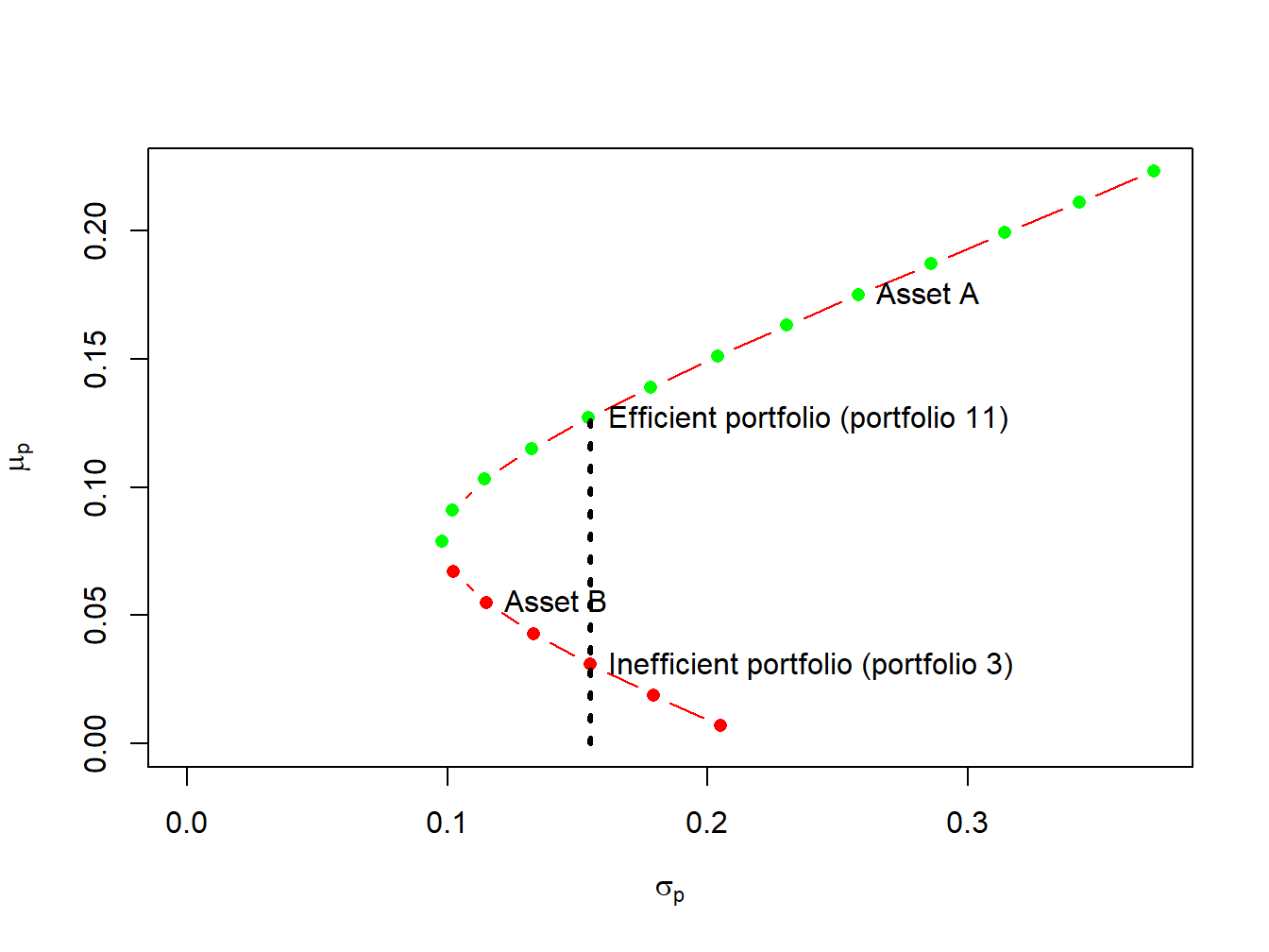
The diagram above depicts both efficient and inefficient portfolios. Efficient portfolios yield the highest expected return for a given standard deviation value. These portfolios are indicated by green dots, commencing with the global minimum variance portfolio situated at the apex of the Markowitz bullet. Inefficient portfolios, marked by red dots, lie below the global minimum variance portfolio. For example, within the diagram, two feasible portfolios, 3 and 11, exhibit identical standard deviation but diverge in expected return values. Portfolio 11, boasting a superior expected return, is categorised as efficient, whereas Portfolio 3, with a lower expected return, is deemed inefficient.

But, how do we find the portfolio with the minimum global variance?

Global Variance Minimum Portfolio

Firstly, we need to determine the optimal values for \(w_{A}\) and \(w_{B}\) that solve the following optimisation problem:

\begin{align} min \ \ \ \ \ w_{A}^2\sigma_{A}^2 + w_{B}^2\sigma_{B}^2 + 2w_{A}w_{B}\sigma_{AB} \end{align}

\(\qquad\) \(\qquad \qquad \qquad \qquad \qquad s.t\)

\begin{align} w_{A} + w_{B} = 1 \end{align}

So, to find the portfolio with the minimum global variance, we need to solve an optimisation problem defined as follows:

What are the values of \(w_{A}\) and \(w_{B}\) that minimise the risk of a portfolio, given by the variance, while ensuring that the sum of these weights is equal to 1?

Note also that the absence of the constraint \(w_{A} + w_{B} = 1\) would simply imply assigning \(w_{A} = w_{B} = 0\), resulting in the minimum possible variance. Thus, we would then encounter what is known as an unrestricted problem. However, assigning \(w_{A} = w_{B} = 0\) does not satisfy our constraint because we are dealing with a constrained problem. In general and at a high-level formalisation, we can solve this problem using Lagrange multipliers.

The constraint \(w_{A} + w_{B} = 1\) is rewritten in homogeneous form:

\[w_{A} + w_{B} = 1 \Rightarrow w_{A} + w_{B} -1 = 0\]

Next, we create the Lagrangian function:

\[L(w_{A}, w_{B}, \lambda) = w_{A}^2\sigma_{A}^2 + w_{B}^2\sigma_{B}^2 + 2w_{A}w_{B}\sigma_{AB} + \lambda(w_{a}+w_{B}-1)\]

We must then minimize this function with respect to \(w_{A}\), \(w_{B}\) e \(\lambda\):

\[\frac{\partial}{\partial w_{A}} = 2w_{A}\sigma^2_{A} + 2w_{B}\sigma_{AB} + \lambda = 0\] \[\frac{\partial}{\partial w_{B}} = 2w_{B}\sigma^2_{B} + 2w_{A}\sigma_{AB} + \lambda = 0\] \[\frac{\partial}{\partial \lambda} = w_{A} + w_{B} - 1 = 0\]

Thus, we obtain the following system:

\[\frac{\partial L(w_{A},w_{B},\lambda)}{\partial w_{A}} = 2w_{A}\sigma^2_{A} + 2w_{B}\sigma_{AB} + \lambda = 0\] \[\frac{\partial L(w_{A},w_{B},\lambda)}{\partial w_{B}} = 2w_{B}\sigma^2_{B} + 2w_{A}\sigma_{AB} + \lambda = 0\] \[\frac{\partial L(w_{A},w_{B},\lambda)}{\partial \lambda} = w_{A} + w_{B} - 1 = 0\]

Representing the system in matrix notation and performing some operations, we find the optimal weight that minimizes the variance:

\[w^*_{A} = \frac{\sigma^2_{B} - \sigma_{AB}}{\sigma^2_{A} + \sigma^2_{B} + 2 \sigma_{AB}}, \ \ \ w^*_{B}=1-w^*_{A}\]

Using the previously presented data, we have:

\[w^*_{A} = \frac{0.01323 - (-0.004866)}{0.06656 + 0.01323 - 2(-0.004866)} = \textbf{0.2021}, \ \ \ w^*_{B} = \textbf{0.7979}\]

Therefore, the expected return, variance, and standard deviation of the portfolio are:

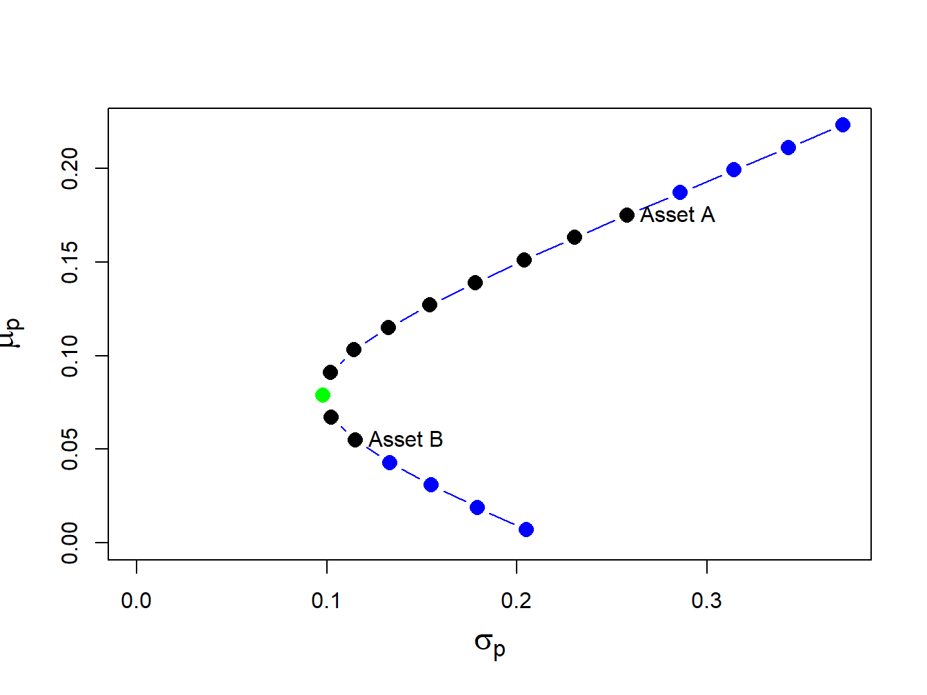
\(\qquad \mu_{p} = (0.2021) \times (0.175) + (0.0.7979) \times (0.055) = \textbf{0.07925}\) \(\qquad \sigma^2_{p} = (0.2021)^2 \times (0.067) + (0.7979)^2 \times (0.013) + 2 \times (0.2021)(0.7979)(-0.004875) = 0.00975\) \(\qquad \sigma_{p} = \sqrt{0.00975} = \textbf{0.09782}\)

In the figure below, the green dot represents the global minimum variance portfolio.

minimum-global-efficient-portfolio

The main feature of this parable is the relationship between assets A and B, indicating their inter-correlation. The fundamental premise of MPT aims to encourage diversification by blending portfolio assets that are not closely correlated, in order to diminish portfolio risk (variance) without compromising returns.

What are the benefits of diversification?

The role of Diversification

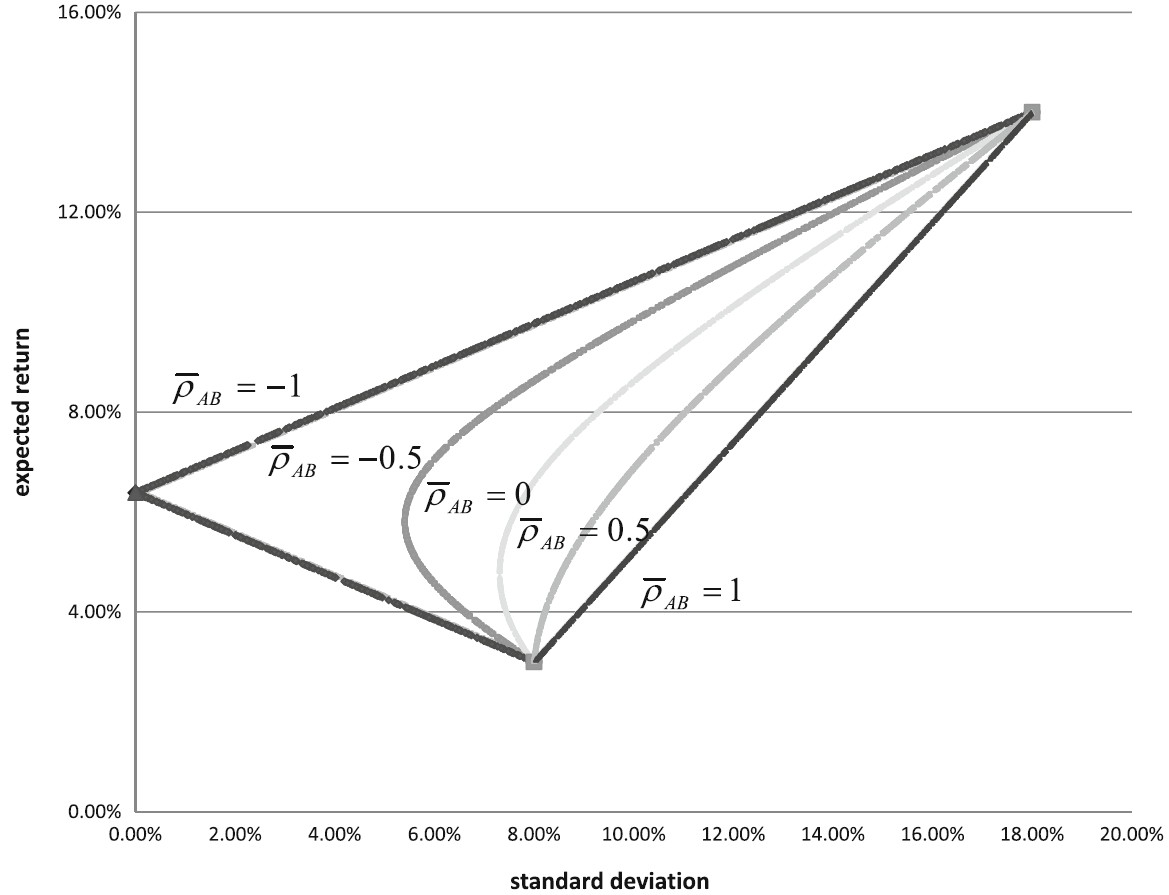
The variance depends on the individual variances of the asset rates of return and on their correlation. For given values of \(w_{A}\) and \(w_{B}\) Eq. (1.8) shows that the variance of the portfolio rate of return decreases when decreasing \(\rho_{AB}\) from \(1\) to \(-1\).

The variance is influenced by the individual variances of the asset returns and their correlation. For given values of \(w_{A}\) and \(w_{B}\) the variance of the portfolio return decreases as the correlation \(\rho_{AB}\) decreases from \(1\) to \(-1\)

The variance is affected by both the individual variances of the asset returns and their correlation. With fixed values of \(w_{A}\) and \(w_{B}\), the portfolio return’s variance decreases as the correlation \(\rho_{AB}\) decreases from \(1\) to \(-1\)

Let’s examine the extreme cases:

\(\overline{\rho}_{AB}\) = 1: When the assets are perfectly positively correlated, the frontier becomes a straight line connecting the points corresponding to portfolios comprising of each asset individually. The frontier comprises deviations of the two assets, with coefficients \(w_{A}\) and \(w_{B}\), \(w_{A} + w_{B} = 1\).

\[\sigma^2(x) = w_{A}^2\sigma_{A}^2 + w_{B}^2\sigma_{B}^2 + 2w_{A}w_{B}\sigma_{AB} = (\sigma_{A}w_{A} + \sigma_{B}w_{B})^2\]

In this case, the portfolio’s standard deviation is a convex combination of the standard deviations of the two assets, with coefficients \(w_{A}\) and \(w_{B}\), \(w_{A} + w_{B} = 1\).

\(\overline{\rho}_{AB}\) = -1: When assets are perfectly negatively correlated, the frontier comprises two intersecting lines on the expected return axis (zero standard deviation). This phenomenon can be elucidated by examining the following formula:

\[\sigma^2(x) = w_{A}^2\sigma_{A}^2 + w_{B}^2\sigma_{B}^2 + 2w_{A}w_{B}\sigma_{AB} = (\sigma_{A}w_{A} - \sigma_{B}w_{B})^2\]

Since \(w_{B} = 1 - w_{A}\), the standard deviation \(\sigma_{A}w_{A} - \sigma_{B}w_{B}\) becomes null when \(w_{A} = \frac{\sigma_{B}}{\sigma_{A} + \sigma_{B}}\). For values of \(w_{A}\) lower and greater than \(\frac{\sigma_{B}}{\sigma_{A} + \sigma_{B}}\) two straight lines are obtained.

correlation-plot

Now consider \(N\) uncorrelated assets with the same expected return and variance.

\[E[R_{i}] = 0.2\] \[\sigma^2_{i} = 1\] \[cov(i,j) = 0 \ \ \forall \ \ i \neq j\]

If we invest all resources in just one of the assets, then the portfolio performance will be \((R_{p} , \sigma^2_{p}) = (0.2, 1)\), which represents the return and variance, respectively. Now, consider a portfolio with \(N\) assets and weights \(W_{i} = 1/N\). The expected return of the portfolio equals that of its components.

\[\mu_{p} = \sum_{i=1}^{N}\frac{1}{N} \times 0.2 = 0.2\]

However, the variance is given by:

\[\sigma^2_{p} = \sum_{i=1}^{N}\frac{1}{N^2} \times 1 = \frac{N}{N^2} = \frac{1}{N}\]

where \(N\) is the number of assets in the portfolio.

Note that the variance tends towards zero as \(N\) increases, and the portfolio becomes risk-free, assuming that the assets are uncorrelated, which in practice is very unlikely to happen - In reality, there is always correlation between assets. Generalizing the model proposed by Markowitz, let’s assume that there are \(N\) assets that can be part of the portfolio, with expected returns \(M_{i} = E[R_{i}]\) and covariance \(\sigma_{ij}\) for \(i\), \(j=1,2,...,N\). A portfolio is then defined by a set of weights \(W = \{ w_{1},...,w_{n}\}\) onde \(w_{1} +...+ w_{n} = 1\). Thus, the general model proposed by Markowitz to find the portfolio of minimum variance is given by:

\[\sigma^2_{p} = \sum_{i=1}^{N}\sum_{j=1}^{N}w_{i}w_{j}\sigma_{ij}\]

\(\qquad \qquad \qquad \qquad \qquad \qquad\) s.t

\[\sum_{i=1}^{N}w_{i}=1\]

Note: A subtle change is to consider \(j+1\) in the minimization to only contemplate the upper triangular part.

Also note that

\[\sum_{i=1}^{N}\sum_{j=1}^{N}w_{i}w_{j}\sigma_{ij} = \sum_{i=1}^{N}\sum_{j=1}^{N}w^2_{i}\sigma^2_{i} + 2\sum_{i=1}^{N-1}\sum_{j=i+1}^{N}w_{i}\sigma_{i}\]

where:

\(\sum_{i=1}^{N}\sum_{j=1}^{N}w_{i}\sigma^2_{i}\) it is the sum of the squared weights times the squared variance.
\(2\sum_{i=1}^{N-1}\sum_{j=i+1}^{N}w_{i}\sigma_{i}\) It is twice the weight of \(i\) times the weight of \(i\) times the weight of \(j\) times their covariance for all pairs.

The system above can be solved using Lagrange multipliers, where we then have a system with \(N+1\) equations and \(N + 1\) variables. The variables are given by \(w_{1,...,w_{N}}\) and \(\lambda\) and the \(N+1\) equations are the partial derivatives with respect to each of the weights and with respect to \(\lambda\) as we did in the previous section. The above model is referred to as a** Quadratic Programming** model with linear constraints.

Portfolio Optimization Process (Bonus)

When defining the optimization framework, timing becomes a crucial factor that requires careful consideration. There’s a specific point in time when the portfolio is initially constructed, and assets are purchased, which is referred to as the investment time. Subsequently, there may be occasions when the existing portfolio undergoes revisions and adjustments to accommodate market changes. During such times, assets may be bought or sold.

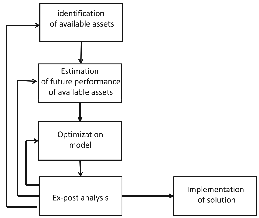
The optimization process typically involves several key steps:

Gathering information, beliefs, and methods to estimate the performance of available assets at the target time.
Selecting a model that, based on the estimations obtained in the previous phase, generates a portfolio.
Assessing the model through ex-post analysis and providing possible feedback to one of the previous phases.
Implementing the portfolio.

Portfolio Optmization Process

Measuring the past performance of a portfolio against a benchmark is relatively straightforward using its rate of return, including potential dividends. However, ensuring the future performance of a portfolio is a more challenging task. The expected return of a portfolio over a certain period should not be a single measure for an asset or portfolio. The rate of return of an asset over a certain period can be modeled as a random variable, and consequently, the rate of return of a specific portfolio is also a random variable.

The performance issue relates to the trade-off between the expected value of the uncertain rate of return of a portfolio and its level of variability. Variability should measure the associated risk, the risk of not achieving what is expected. Typically, a high expected return cannot be achieved without a high level of risk. The selection of a specific trade-off level, such as between a portfolio with high return and high risk and one with low return and low risk, can only be made by the investor. Risk aversion will lead an investor to prefer the latter over the former, while risk propensity will lead to the former over the latter.

Conclusion

To conclude, the Markowitz model epitomizes the fusion of mathematics and finance, providing investors with a potential instrument to enhance their portfolios in an unpredictable environment, and although the model’s mathematical foundations may seem complex initially, its fundamental principles are rooted in intuitive concepts that resonate with investors globally.

As we explore the complexities of the Markowitz model, it becomes clear that its robustness stems not just from its mathematical precision but also from its capacity to adjust to real-world investment situations. Despite criticisms highlighting its assumptions’ limitations, the model’s continued relevance highlights its importance as a guiding principle for wise investment decision-making. Despite that, It is evident that the portfolio optimization methods employed in the financial industry are based on assumptions that do not align well with the real world. As we strive to deepen our understanding of financial markets, the Markowitz model endures yet in a constantly evolving landscape.

However, these tools are often used and trusted by individual investors and advisers as if the underlying assumptions were accurate. As I read from an economist statement: Within the models, there are no flaws. The flaws lie in the assumptions.

Final Thoughts

If you’ve read this post so far, thank you very much, I hope this material has been useful and makes sense to you, and if any other topic related or not to the content of this post interests you, or has left you in doubt, put it in the comments and I will be very happy to bring the content more clearly in a new post.

Remembering that any feedback, whether positive or negative, just get in touch via my twiter, linkedin, Github or in the comments below. Thanks.

References

[1] Markowitz, H. M. (1952). Portfolio selection. Journal of Finance 7, 1: 77–91
[2] Foundations of Portfolio Theory
[3] Benninga, S. 2000. Financial Modeling. Second Edition. Cambridge, MA: MIT Press.
[4] Bodie, Z., A. Kane, and A. J. Marcus. 2013. Investments. 10th Edition. McGraw-Hill Education.
[6] Markowitz, H. 1959. Portfolio Selection: Efficient Diversification of Investments. New York: Wiley.
[8] Portfolio Optimization Theory Versus Practice
[9] Linear and Mixed Integer Programming for Portfolio Optimization